Previous chapters in this thesis described methods to optimize Earth Observations (EO) of the hydrologic cycle. These methods make adjustments to EO datasets so that they can be combined to create a balanced water budget. In the preceding chapter, I described how the models were applied at the pixel scale to create calibrated EO datasets with higher hydrological coherency than the uncorrected EO datasets.
In this chapter, I show how these calibrated EO data can be used to make improved predictions over ungaged or un-instrumented basins. For example, we may estimate runoff in ungaged basins or calculate total water storage change (TWSC, or ΔS) to fill in missing GRACE satellite observations. This opens up a number of possibilities for using the model-calibrated EO data. Water budget-based approaches can be used to estimate any one of the four components based on the other three, by rearranging the terms of the water balance equation, \(P - E - \Delta S - R = 0\). This is an important application of the calibrated database. It can be seen too as an additional way of evaluating the calibrated data. As we will see below, many researchers have applied this method with remote sensing data, with varying degrees of success.
The water budget approach is applied to estimate evapotranspiration, E, runoff, R, and total water storage change, TWSC or ΔS. (I did not attempt to calculate P by inference, as this variable is already calibrated to a large set of rain gages, and the model is unlikely to be useful for prediction.) My hypothesis was that estimating missing water cycle components via this method could be improved by using EO data that has been calibrated by the neural network (NN) model described in Chapters 4 and 5. I compared inferred predictions to observations and to the results from other modeling studies. This analysis can help to verify that the models are actually improving EO datasets. Are the predictions a better fit to observations? Are estimates an improvement over using uncorrected EO datasets?
The goodness of fit to observations is often modest, but I found that the fit is greatly improved when using NN-calibrated datasets rather than the original, uncorrected data. The significant improvement in predicting water cycle components with remote sensing data illustrates the usefulness and practical application of the methods described in this thesis.
Prior to GRACE, hydrologists used water budgets as one method of estimating long-term evapotranspiration over river basins. To do so, they assume that there is no trend in total water storage. When this is the case, then \(\bar{E} = \bar{P} - \bar{R}\) over sufficiently long time scales (Lopez, McCabe, and Houborg 2015). A common practice in the northern hemisphere is to perform such calculations over a water year, from October 1 - September 30. However, observations from GRACE have shown that water storage in many regions is dynamic, and can vary significantly over annual and decadal time scales (Rodell et al. 2018). Therefore, the assumption that basin water storage is constant over long time scales appears to be invalid more often than previously thought (see Section 2.7.2). Several recent studies have made use of GRACE data and the water-budget method to estimate evapotranspiration, using \(E = P - \Delta S - R\).
Rodell et al. (2011) estimated E over seven large river basins and compared predictions to the output of several land surface and atmospheric models. They concluded that the uncertainty in GRACE ΔS is too high to produce useful monthly estimates, but that the method produces viable annual estimates of E.
Long, Longuevergne, and Scanlon (2014) estimated E over river basins in Texas using GRACE data, observed runoff, and a variety of data sources for precipitation. The fit of predicted E was modest, with R² ranging from 0.21 to 0.64. Pascolini-Campbell, Reager, and Fisher (2020) estimated monthly basin-scale E over 11 major river basins in the contiguous United States. The authors compared the results of what they called the “mass conservation ET estimate” to E from remote sensing data products and land surface models. They found that using this method and GRACE data consistently reproduced the seasonal pattern of E, but also resulted in higher estimates of E compared to other data sources. Yet, because this study did not include comparison to in situ observations, it is difficult to say which method is the best fit to observations, and hence the most accurate.
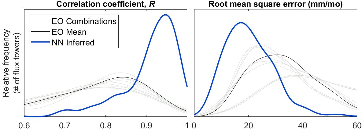
I calculated E by the water budget method with uncorrected EO datasets, then repeated the analysis with NN-calibrated EO datasets. I compared the results to E observed at 117 flux towers across the globe. The results of this analysis are shown in Figure 6.1.
Fit statistics in in Table 6.1 compare the time series of E observed at the tower to the time series from the corresponding grid cell in the calibrated EO data layer of E. Calculating E from uncorrected EO data results in a relatively poor fit. Among the 27 possible combinations, shown in gray on Figure 6.1, the correlation, R, has a mean and standard deviation of 0.64 ± 0.31. The quality of predictions varies depending on which EO database is used as input. Simply averaging multiple datasets has a slight positive effect. The NN calibration further helps improve the fit. Using the NN-corrected EO data to compute E improves the fit, with average R = 0.87.
For the sake of comparison I have also included direct estimates of E in Table 6.1. These appear at the top, under the heading EO datasets. This allows us to see how the water-budget method compares to direct estimates by remote sensing. When we use uncorrected EO data as inputs, it is much less accurate to estimate evapotranspiration by \(E = P - \Delta S -R\). However, after NN calibration, the quality of water budget-based estimates rivals GLEAM or ERA5.
So, the calibration the EO datasets with the NN model allows us to make much more accurate predictions of E with the water budget method, compared to using uncorrected EO data. This shows that the NN-optimization of the water components P, ΔS and R makes them closer to the E in situ measurements. The results appear to be just as good as those obtained with current state-of-the-art remote sensing datasets. They also appear to be better than results reported in several recent studies cited above.
Table 6.1: Goodness of fit to evapotranspiration estimated by various methods, compared to observations at at 117 flux towers. Table entries are the median for the fit statistic over the sample. For EO combinations, table reports the median of the medians.
| Corr. R |
RMSE mm/mo |
Bias mm/mo |
|
|---|---|---|---|
| EO datasets | |||
| GLEAM-A | 0.91 | 21 | 2.0 |
| GLEAM-B | 0.93 | 20 | 2.5 |
| ERA5 | 0.91 | 20 | 3.9 |
| NN mixture model (this study) | 0.92 | 19 | 2.1 |
| E estimated indirectly using | |||
| EO Combinations (n=27) | 0.75 | 34 | 8.1 |
| EO Mean | 0.78 | 32 | 11 |
| NN calibrated EO (this study) | 0.92 | 19 | 0.3 |
We have seen how observations of TWS from GRACE contributed to more holistic study of water cycle. Previously, water storage could only be inferred or estimated indirectly. We have also seen that GRACE data has significant gaps (Section 2.4.1). There is also interest in reconstructing GRACE-like total water storage for periods prior to 2002, using a variety of methods.
F. W. Landerer and Swenson (2012) discuss the difficulty in comparing GRACE observations to the results of simulation models. GRACE TWS does not map directly to a state variables in land surface models, which many not fully simulate groundwater, glaciers, etc. or their simultation may be unrealistic “due to missing model physics” (F. W. Landerer and Swenson 2012). Nevertheless, studies have found that GRACE estimates of TWSC are correlated with observed groundwater surface elevation changes (Rodell et al. 2018), soil moisture estimated by a land surface model (B. R. Scanlon et al. 2019), surface water extent (Papa et al. 2008), and reservoir volume (X. Wang et al. 2011).
B. R. Scanlon et al. (2019) assessed the correlation between GRACE observations and modeled water storage over 183 global river basins, using data from 7 global hydrologic and land surface models. For most of the models they considered, the researchers used the model estimates of soil moisture as a proxy for TWS. The authors concluded that discrepancies between observations and simulations are partly due to missing storage compartments in models (e.g., surface water and/or groundwater). In one of the more thorough analyses conducted to date, Biancamaria et al. (2019) compared observed TWS anomaly to modeled water storage from two hydrologic models in the Garonne river basin in France, and found correlation coefficients of around 0.9 and Nash-Sutcliffe Efficiency of around 0.7.
In another example, Lehmann, Vishwakarma, and Bamber (2022) estimated ΔS by the water budget method over 189 large river basins, and compared predictions to GRACE observations. Rather than seeking to optimize the datasets, the authors looked for the best combination of inputs. The authors deemed their method successful because the Nash-Sutcliffe Efficiency, NSE > 0 in the majority of basins, which means that the model performed better than a constant at the mean of observations. This modest performance underscores the difficulty of estimating TWS based on other, unrelated, remote sensing observations.
Due to the lack of in situ data, I also evaluated the results of my NN model against results from other studies that predicted GRACE-like total water storage change using different methods, including those that were more sophisticated than the simple water balance method used here. Pan et al. (2012) estimated the water budget components using satellite observations in 32 globally distributed major basins for 1984–2006. Their approach used data assimilation techniques, first estimating the errors in each water budget component by comparison to in situ observations, then using a constrained Kalman filter to merge the datasets based on their error information, with a goal of minimizing the imbalance. Yu Zhang et al. (2018) employed a similar method at the pixel scale, rather than at the scale of the river basin. The authors concluded that the imbalance error is mainly due to disagreement among evapotranspiration estimates.
I obtained the results from Pan et al. (2012) by request to the author, and downloaded the data from Yu Zhang et al. (2018). I used geodata for Pan’s 32 large basins (basin masks on a 1° grid) to calculate the spatial-averaged means for changes in storage over these basins. Because Zhang et al. produced global gridded estimates of TWSC, I could compare the results to GRACE observed TWSC at the pixel scale. For my NN model and Zhang’s model, I averaged the estimated TWSC over the 32 large river basins used in Pan’s study. Pan et al. (2012) includes data for the years 2000 - 2006, while Yu Zhang et al. (2018) covered 1984 - 2010.
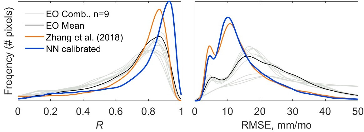
Overall, ΔS predicted by the water-budget method using NN-calibrated EO data was a better fit to GRACE observed ΔS, according to two common goodness-of-fit measures (Figure 6.2). On these plots, the blue points represent the fit indicator in one basin, and the red line is the median. I compared the model fit to the simple-weighted average of the three GRACE solutions for TWS. These results are also reported in Table 6.2
Over these 32 large basins, Pan’s model had a median correlation coefficient R = 0.86, compared to Zhang’s R = 0.90, and R = 0.94 for my model. Pan’s model had a median root mean square error, RMSE = 12.0, compared to RMSE = 10.2 for Zhang’s model, and RMSE = 8.0 for my model. Thus, in these large river basins, my NN model is a better fit to GRACE observed TWSC. The comparison may not be entirely fair, as I have calibrated my NN model using recently published versions of GRACE, while Pan’s model was calibrated to an older version of GRACE available in 2012.
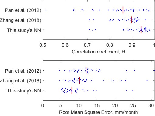
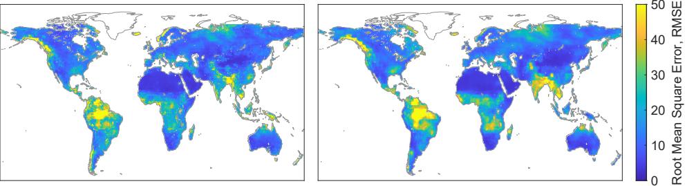
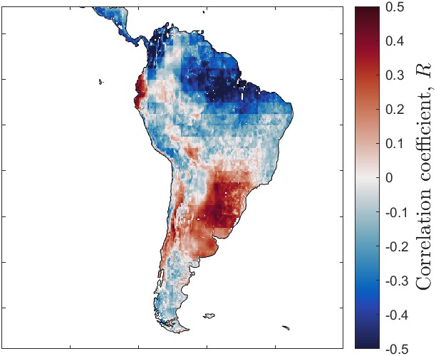
Figure 6.3 shows the fit to observed TWSC by my neural network model and the predictions by Yu Zhang et al. (2018). The map shows that the geographic patterns are similar, in terms of where the models produce better or worse fits to observations. Overall, my model has a slightly higher median correlation with observations, and a slightly lower root mean square error. However, my model performs poorly in more geographic areas.
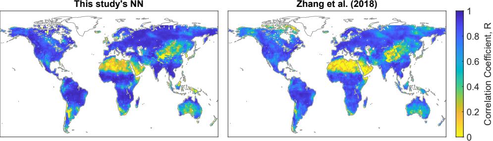
The results in Table 6.2 show that our model’s indirect estimates of ΔS are equivalent to the predictions by Yu Zhang et al. (2018), based on the fit to GRACE observations at the pixel scale over the overlapping time period 2002 to 2009. It was not among the main goals of this research to predict TWSC. Nevertheless, my NN model is able to do so nearly as well as a state-of-the-art model.
Table 6.2 Goodness of fit to GRACE observations for total water storage change estimated indirectly by the water-budget method, in 57,286 land pixels. Table entries are the median for the fit statistic over the sample. For EO combinations, table reports the median of the medians.
| TWSC, ΔS, estimated indirectly by | Corr. R |
RMSE mm/mo |
Bias mm/mo |
|---|---|---|---|
| EO combinations (n=9) | 0.71 | 24 | 3.3 |
| EO Mean | 0.75 | 22 | 6.4 |
| Zhang et al. (2018) | 0.79 | 13 | 0.09 |
| NN calibrated EO (this study) | 0.84 | 13 | 0.18 |
At the pixel scale, the results of my NN predicted ΔS compare favorably to those predicted by Zhang. Figure 6.4 shows the empirical probability distribution for two fit indicators over land pixels. (This figure visually summarizes the same data as Table 6.2.) The average correlation for Zhang is R = 0.70, while for my model, R = 0.74. My NN model’s median correlation is slightly higher, with median R = 0.84 vs. Zhang’s median R = 0.79.
A limitation of the water-budget method for estimating TWSC is that its inputs are hydroclimatic variables only. It does not include information on human influence on the water cycle, such as groundwater pumping, irrigation, withdrawals, or interbasin transfers. Because of this, these methods will be less accurate in zones with extensive human impacts. In zones without anthropogenic influences, the results may help show how water storage responds to climate and meteorological forcing.
Using the methods above, I reconstructed a signal of Total Water Storage Change, ΔS for the period 1982 - 2019, which includes 20 years prior to the launch of the GRACE satellites. In the section above, I showed that the reconstruction is a reasonably good fit to observations. It is interesting to examine the relationship between water storage and other climate variables. Since the late 19th century, scientists have “teleconnections” in weather and climate – the relationships or links between phenomena at widely separated locations of the globe.
Studies have used various methods to identify and analyze teleconnections in hydrology. For example, Martens et al. (2018) highlighted the need to consider teleconnections to accurately predict the fate of the terrestrial branch of the hydrological cycle. They used observational evidence to improve the representation of surface fluxes in Earth system models. Similarly, Rasouli et al. (2020) conducted variance, correlation, and singular spectrum analyses to identify hydroclimatic phases related to teleconnection patterns in a small headwater basin in Idaho, USA. Their study linked hydrological variations at local scales to regional climate teleconnection patterns.
With a nearly 40-year reconstruction of ΔS, it is interesting to analyze the relationship between water storage and well-known climate patterns. The El Niño Southern Oscillation (ENSO) is a quasi-periodic climate pattern that characterizes the warming and cooling of surface waters in the eastern tropical Pacific Ocean (El Niño) and its effect on air pressure across the equatorial Pacific Ocean (Southern Oscillation). During El Niño events, there is a warming of the ocean surface temperatures in the central and eastern Pacific, causing changes in atmospheric circulation and rainfall patterns experienced across the globe (Guimarães Nobre et al. 2019).
The ENSO cycle consists of two phases: El Niño and La Niña. For example, in South America, El Niño, there is often increased rainfall along the west coast of South America, leading to increased flooding and landslides. In North America, El Niño can bring above average precipitation in the southern United States, and drier than average conditions to parts of the Pacific Northwest. In Australia and Southeast Asia, El Niño is linked to reduced rainfall and drought. It is also linked to increased rainfall in parts of eastern Africa, while in India, El Niño is associated with reduced precipitation.
I downloaded ENSO indices from the NOAA (2023) and analyzed the correlation with my reconstructed 38-year dataset of TWSC. There are several different ENSO indices available, based on different variables, and calculated over different regions of the Pacific Ocean. I based the analysis here on the Multivariate El Niño/Southern Oscillation (ENSO) index (MEI.v2) index, which combines “five different variables (sea level pressure (SLP), sea surface temperature (SST), zonal and meridional components of the surface wind, and outgoing longwave radiation (OLR)) over the tropical Pacific basin (30°S to 30°N and 100°E to 70°W).”
The relationship we see here is consistent with what we know about how El Niño events can affect weather patterns and the water cycle in different parts of the world. Figure 6.5 shows the correlation between TWSC with the ENSO index MEIv2 over South America. The temporal behavior is also coherent with correlations positive or negative up to 0.5. The interpretation is that ENSO can explain up to 25% of the variability in the monthly TWSC.
One interesting application of the extended reconstruction of TWSC is to analyze trends. Reconstructing the signal of TWSC was not my main goal. However, combining the water budget method with NN-calibrated EO data allows us to reconstruct the signal of ΔS about as well as a state-of-the-art assimilation model. However, challenges remain in terms of reconstructing TWS. The variable predicted by my model, ΔS, is a change in the volume of water stored over time, in units of mm/month. Water managers are usually more interested in the time integral of this rate, or the total water storage, TWS. When I calculated this quantity by integrating ΔS, I found that even relatively small errors or biases in the signal of TWSC are compounded when calculating the integral, causing unacceptably large uncertainties.
It can be shown that any slight inaccuracies or biases in ΔS are magnified when integrating to determine S, the total water storage. Thus, the estimates of the trend are highly uncertain. I do not believe that any of the current published reconstructions of GRACE-like water storage are sufficiently accurate to reliably estimate trends in water storage in the pre-GRACE era. This makes it difficult to reliably calculate trends in TWS given a reconstructed signal of TWSC. Thus, it is possible to use my NN model, or the other models described above, for hindcasting, or to make predictions of TWSC for before the GRACE satellites were launched in 2002. We can adequately reproduce the seasonal pattern, but it is impossible to accurately predict trends. Therefore, the usefulness of these predictions is severely limited.
For future research, there are certain strategies which may help to produce more robust reconstructions of TWSC, which could help improve the estimation of trends. One strategy is to combine both observed and modeled time series of ΔS to estimate the trend, using Bayesian estimation or Kalman filters. One could also try debiasing modeling results to fit the observations before using them to estimate the trend, e.g., with CDF matching, or quantile-quantile bias correction. However, I believe that trends in water storage estimated using climate data will always be suspect if they do not include human influences such as diversions and withdrawals, which have a major impact on the water cycle in many locations.
Considering the decline in river discharge monitoring in recent decades, alternative methods of estimating runoff are becoming more important. As we have done above with E and ΔS, we may use the water budget approach to predict runoff, R, from the other three water cycle components. Lorenz et al. (2014) refers to this method of estimating basin-scale runoff as the “hydrologic approach.” One of the main advantages of this approach is that it “does not require runoff routing as it is taken care of by the water storage changes.”
Researchers have largely been unsuccessful in trying to estimate river discharge using such water-budget based methods. Frequently, the magnitude of runoff is small compared to the other components, making the signal-to-noise ratio low. And, as noted by Lorenz et al. (2014), “the accuracy of the runoff estimates will be only as good as the least accurate dataset.” Despite these difficulties, predicting basin runoff by indirect methods is a compelling topic of research. Developing a new, accurate method for prediction in ungaged basins would be considered a major breakthrough. Such predictions would be highly valuable in regions with limited measurement infrastructure, with potential applications in agricultural water management, drought and famine prediction, or predicting the impacts of climate change on future runoff (Chiew 2010).
Some authors have made the simplifying assumption that, over sufficiently long time periods, \(\Delta S = 0\) (i.e. no trend in storage), allowing one to estimate long-term average runoff as \(R = P - E\) (Y. Liu et al. 2020). There are several recent studies where the authors use data from GRACE to provide this information. Syed et al. (2005) used GRACE data and P and E from a reanalysis model to estimate discharge over the Mississippi and Amazon basins. Overall, the fit was poor, and prediction errors were high. Nevertheless, the authors expressed confidence in the method, and hypothesized that observed discharge at gages may not adequately capture the flux out of the basin, which may be exiting via subsurface flow and other “unmonitored surface fluxes.”
Sheffield et al. (2009) used GRACE and other remote sensing data to impute the discharge from the Mississippi River basin. Their results were fairly poor – the 95% confidence interval for estimated discharge in certain months ranged from −3 to +3 mm/day, equivalent to a range of −100,000 to +100,000 m³/s. (The mean discharge of the Mississippi at Vicksburg is around 16,000 m³/s.)
Gao et al. (2010) used the water budget method to infer runoff over 9 large river basins in the continental United States. The predictions also appear to be rather poor; while the authors do not report any fit statistics, simply noting that errors are “generally quite large, especially during the warm season.”
Lorenz et al. (2014) used EO data to predict runoff over 96 global river basins ranging in sizes from 20,000 km² to 4 million km² (the Amazon). The authors concluded concluded that “the budget-based approaches do not provide realistic runoff estimates because of significant biases in the input datasets.” The water budget-based model performed worse in river basins where the flows are low or nearly constant. Sneeuw et al. (2014) attempted to estimate river discharge using the same method, which they called “the hydrogeodetic approach,” over 5 large river basins. The results were again relatively poor, with NSE > 0 (meaning the model outperforms the mean of observations, \(f(x) = \bar{x}\)) in only 1 of the 5 basins. The authors expressed the hope that better runoff predictions would be possible in the future after “improvements in the quality of global hydrological and hydro-meteorological datasets.”
J. Chen et al. (2020) estimated river runoff in the Amazon basin using data from GRACE, ERA5 reanalysis data, and satellite precipitation observations for 2003 through 2015. Their water-budget based estimates of runoff exceeded observations by about 30%. The authors speculate that there is a significant subsurface runoff flux that contributes in part to this difference. Indeed, there is evidence of significant groundwater flow in the aquifer beneath the Amazon, equivalent to around 3% of river flow (Pimentel and Hamza 2011). However, this subsurface flow only accounts for about 1/3 of the difference between observed flow and estimates by J. Chen et al. (2020).
In a more recent paper, Abolafia-Rosenzweig et al. (2021) predicted discharge over 24 global basins combining remote sensing and in situ observations. The authors concluded that they were not able to accurately predict discharge (R² ranged from 0.42 to 0.47), concluding that the uncertainties in other water budget components are “generally larger than the magnitude of \(Q\) [discharge] itself.” However, the authors also found that adding the water cycle closure constraint contributed to improved predictions of discharge.
For this analysis, I calculated R indirectly using the three NN-calibrated water cycle components. The output is a gridded data layer of R at the pixel scale. We may then compute the spatial average to estimate river discharge in small- to mid-size river basins. Figure 6.6 and Table 6.3 compares the fit to observations of runoff calculated by inference from uncorrected remote sensing datasets, and by the calibrated EO data output by my NN model. The NN-based result is a significant improvement over using uncorrected EO data.
The uncertainty in runoff estimated by the water budget method is too high to consider this a reliable estimator of discharge in un-gaged basins. This is a signal-to-noise ratio issue. Runoff tends to be much smaller in magnitude than the other three water cycle components. However, the coherency between the WC components has been improved by the NN framework.
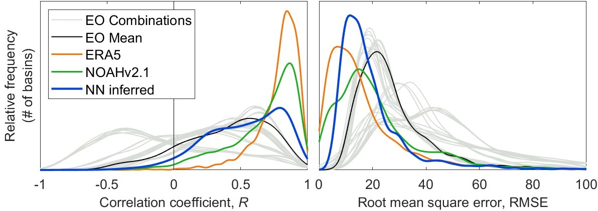
In Figure 6.6, showing the fit to observations for runoff predicted by inference, there is a sub-ensemble in gray with first mode around -0.5. These lines have all been calculated with GLEAM-A. evapotranspiration dataset. Because use of this particular dataset tends to result in poorer predictions of observed runoff, one may choose to discard it in future water cycle analyses. Indeed, the data provider publishes different versions of GLEAM, as described in Section 2.3.2. GLEAM-A uses meteorologic inputs from reanalysis modeling, while GLEAM-B relies more on remote sensing data. In this context, predicting runoff via the water-balance method, GLEAM-A yields larger errors, so preference should be given to GLEAM-B.
Based on the results in Table 6.3, we can see estimated runoff using NN-calibrated EO data has a lower bias error than estimates made with uncorrected EO data. A summary of the percent bias errors over 1,781 river basins is shown in Figure 6.7. Recall that the bias measures the distance between the mean of observations and the mean of predictions. The percent bias is the percentage difference between the means of observations and predictions.
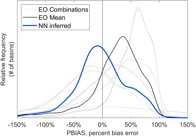
Table 6.3: Goodness of fit between runoff estimated indirectly by the water-budget method and observed river discharge at 1,781 river gages. Table entries are the median for the fit statistic over the sample. For EO combinations, table reports the median of the medians.
| Water cycle component | Corr. R |
RMSE mm/mo |
Bias mm/mo |
|---|---|---|---|
| Modeled Runoff | |||
| GRUN | 0.45 | 21 | 8.2 |
| ERA5 | 0.83 | 13 | 0.5 |
| NOAHv2.1 | 0.76 | 18 | 1.6 |
| Runoff estimated indirectly with | |||
| EO Combinations (n=27) | 0.29 | 31 | 2.4 |
| EO Mean | 0.45 | 24 | 8.2 |
| NN calibrated EO (this study) | 0.57 | 16 | 1.0 |
We saw in Figure 6.6 that inferences of R via the water balance that use the NN-calibrated data are significantly improved compared to using uncorrected EO datasets. Nevertheless, the accuracy of these predictions is still modest, and errors may be too high for many applications. Further, predictions of runoff via a monthly water-balance model would not be suitable for all applications. For example, flood warning would typically require hourly or at least sub-daily temporal resolution. However, such estimates could be useful in agricultural water management or famine early warning systems. I also investigated whether the NN calibration improves estimates of the long term mean of R. Even when the RMSE is too high, information on the mean runoff is still valuable information for prediction over ungaged basins. At least we may say that it provides a first-order estimate of runoff and river discharge.
Based on the simple-weighted average EO data, runoff estimates had a median bias error of -20 mm/month, compared to -3 mm/month using NN-calibrated data. For the sake of this analysis, let us suppose that estimates of discharge are adequate when the absolute value bias error is less than 50% (i.e.: the prediction is within 50% of the truth, regardless of whether the estimate is too high or too low). With uncorrected EO data, the estimated runoff had a bias error less than 50% in 1,022 out of 1,781 basins, or 57% of the time. After NN calibration of EO data, the number of basins where \(\left| \text{PBIAS} \right| < 50\%\) increases to 1,261, or 71% of the total. Based on these statistics and Figure 6.7, we can see that NN calibration leads to a significant improvement of estimates of runoff made via the water-budget method.
As described above, several studies have used water-budget based methods to estimate discharge in large river basins, such as the Amazon and the Mississippi. We saw above that using NN calibrated EO datasets resulted in significant improvements in runoff prediction, compared to using uncorrected EO datasets. I tested the water budget method’s ability to predict discharge in the Mississippi River basin, comparing the results to observations (USGS gage 07289000 at Vicksburg).
Figure 6.5 shows for predicted and observed discharge, with the time series (left) and the monthly average ± standard deviation (right). As can be seen with the light gray lines, R estimated with various combinations of EO datasets varies widely, and is often wildly inaccurate. Discharge estimated with the simple-weighted mean of EO datasets appears to be unbiased during the months of December through May, but exhibits a significant high bias from June to November. Calibrating the EO datasets with the NN model results in improved predictions of basin runoff over the Mississippi.
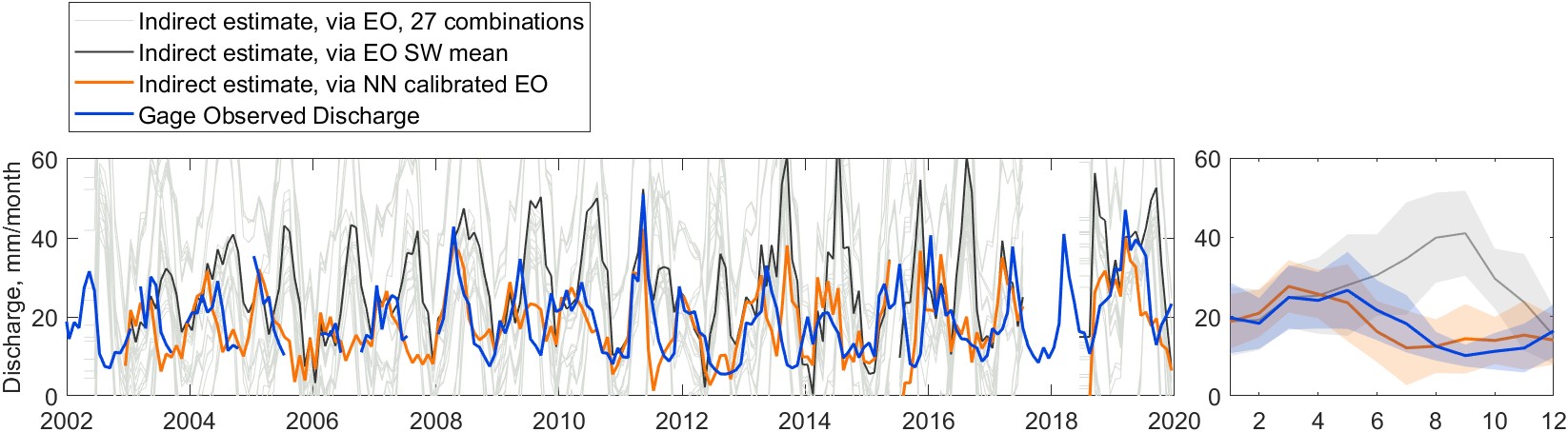
I believe that this result is better than the results in several of the papers cited above that predicted flows in the Mississippi using water-budget based methods. It is hard to say this definitively, as some of these papers describe their results qualitatively, without reporting fit statistics. It is also worth noting that my results are for a longer time period, from 2002 to 2019, with gaps where GRACE data are missing.
Table 6.4: Fit statistics for monthly runoff for the Mississippi River at Vicksburg calculated from EO datasets, pre- and post-calibration by the NN model.
| Pre-calibration | Post-calibration | |
|---|---|---|
| Bias, mm/month | 8.6 | −0.6 |
| RMSE, mm/month | 16.8 | 8.6 |
| Correlation, R | 0.12 | 0.53 |
| KGE | −0.10 | 0.53 |
| NSE | −2.8 | 0.017 |
| CNSE | −4.9 | −0.55 |
Table 6.4 reports several fit statistics comparing predicted discharge with observations, for pre- and post-calibrated EO datasets. Overall, this method is able to predict annual mean discharge quite well, as evidenced by a low bias. The seasonal pattern is also mimicked with good accuracy. However, in terms of a predictive model, this method is not very strong. A Nash-Sutcliffe Efficiency (NSE) near zero means that a constant model equal to the long term mean performs equally well. The Cyclostationary NSE removes the seasonal cycle prior to estimating the goodness of fit. A CNSE < 0 indicates that this method does not do a good job predicting the anomalies.
In this chapter, I applied water-budget based methods for estimating missing water cycle components. With this method, we are solving for one unknown when we have three known variables in the equation \(P - E - \Delta S - R = 0\). This method has been widely used in research and by practitioners.
For evapotranspiration, water-budget based methods predict observed E at flux towers as well as state-of-the-art methods based on remote sensing and more complex models. Indirect water-budget based methods can be used to reconstruct historic TWSC from 1982 to present. However, these results appear to be of relatively low quality. Time series are correlated with climate factors like El Niño, but should not be relied on to estimate trends. Predictions of runoff, while improved, cannot compete with land surface models in terms of predicting river discharge. Overall, this is an important extension of this research, and also an additional way of evaluating the results.
The quality of water-budget based estimates for a missing component is dependent on several factors, including the uncertainty of the 3 inputs variables and the signal to noise ratio. It is, for example, difficult to estimate discharge in basins where the discharge is much less than the precipitation. Yet, the estimation of water cycle components is significantly improved compared to using uncorrected EO data. This is further evidence that the calibrated EO database has greater coherency and better describes the overall water cycle.