Since the beginning of the space age in the 1960s, satellite remote sensing has been used to monitor water on the Earth and in the atmosphere. Today, there are dozens of earth-orbiting satellites collecting data that is translated into estimates of the major components of the water cycle (WC): precipitation, evapotranspiration, and changes in water storage.
The launch of the Gravity Recovery and Climate Experiment (GRACE) satellites in 2002 gave the scientific community the extraordinary capability of monitoring changes in water storage, including in underground aquifers. The twin satellites do this by taking repeated, accurate observations of the Earth’s gravity field. Information on water storage change had long been the “missing link” for calculating accurate water budgets. It is now possible to account for the water in river basins using data from satellite remote sensing plus river discharge from ground-based measurements. River discharge is the only one of the main water cycle components that is not routinely measured from orbit, although this is expected to change with the recent launch of the Surface Water and Ocean Topography (SWOT) mission on December 16, 2022.
The water cycle is an important field of study for earth scientists and for water resources planning and management. Analyses have relevance to drought, floods, agriculture, water supply, and more. And while enormous progress has been made in monitoring the water cycle via remote sensing, capturing a complete picture of the water cycle from space remains challenging.
Despite the many advances in sensor technology and calibration methods, earth observation datasets still have significant errors or biases. Over a decade of research has shown that one cannot “close the water cycle,” or create a balanced water budget using satellite data (Trenberth et al. 2007; Rodell et al. 2015). The usefulness of earth observation (EO) datasets has not been fully achieved because of this “incoherence” among various data products. McCabe et al. (2017) called the ability to monitor (and close) the water cycle “one of the outstanding challenges of hydrological remote sensing.”
The research described in this thesis is an integrated, data-driven approach to balancing the water budget at the global scale using remote sensing data. I am seeking to optimize EO datasets describing the complete hydrologic cycle using statistical methods, without the use of a simulation model. I describe development and application of analytical and modeling methods to “recalibrate” remote sensing data so they result in a balanced water budget.
The methods are rooted in the “ensemble philosophy” – the idea that each dataset can contribute important information. The integrated approach optimizes WC components simultaneously rather than one at a time. In other words, to optimize observed precipitation data, we can make use of information about runoff and evapotranspiration. The premise is that these variables contain useful information for optimizing precipitation, because they are interrelated via the water cycle.
The output of my research is a new, more consistent dataset that quantitatively represents the water cycle over continental land surfaces. This is of scientific interest and practical relevance. The results show where EO datasets are less consistent, and where larger corrections are needed. This information can be used to help evaluate which datasets are best in a particular region, for example for water budgeting or modeling. The results should be of interest to data providers and algorithm developers, “to optimize existing water cycle products or identify deficiencies in current observations” (Dorigo et al. 2021).
For the remainder of this Introduction chapter, I aim to provide the context for this research, drawing from the fields of hydrology and remote sensing. I begin by briefly describing developments within the field of hydrology that have led, in the last few decades, to the era of large scale hydrology, or study of the water cycle at the global scale. I follow with a brief overview of the water cycle and describe the water budgets, a simple but powerful method used everywhere in water science and management. Next, I will give an overview of remote sensing of the water cycle. The treatment is of necessity superficial, as this is a large and diverse field. Finally, I describe various attempts that have been made to close the water cycle through a review of recent literature. These sections provide the background and motivation for my research.
Hydrology is the branch of science concerned with the movement and distribution of water through Earth’s atmosphere, land surface, and subsurface. Some historians credit Leonardo da Vinci as the founder of modern hydrology (Rosbjerg and Rodda 2019). Indeed, he performed pioneering measurements and put forth important ideas. But it was not until centuries later that the modern concept of the water cycle emerged. The French scientist Pierre Perrault performed a detailed accounting of rainfall and river flows of the Seine, described in his 1674 book De l’Origine des Fontaines (On the Origin of Springs). Perrault was the first to describe the water cycle more accurately, “stipulating that inflows to any area of any period of time shall always equal outflows in addition to the change in water storage” (Pfister 2018).
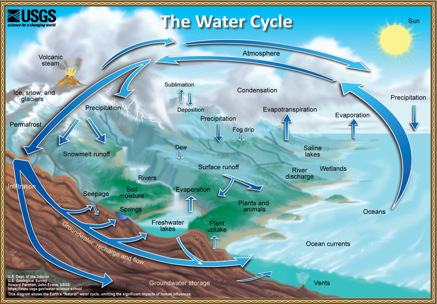
A typical representation of the natural water cycle is shown in Figure 1.1. This familiar version has been critiqued for its failure to show human activities (Abbott et al. 2019), which can have a major influence on the water cycle. Three years after the publication of this critique, the U.S. Geological Survey published a new water cycle diagram that breaks with tradition by showing many human water uses. This new water cycle diagram, shown in Figure 1.2 is a fitting one for our current era, the Anthropocene – the recent geological period during which human activity has been the dominant influence on climate and the environment.
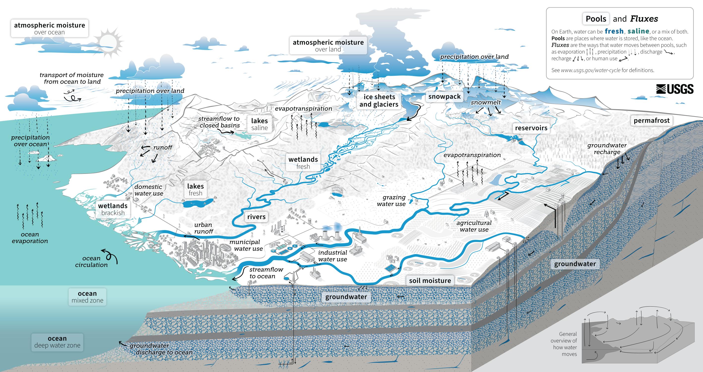
The water cycle diagram in Figure 1.2 includes another important innovation. It accurately reflects the conceptual model used by scientists and engineers by showing pools and fluxes. A pool is a volume of water stored in a particular zone, such as atmospheric water vapor, soil moisture or groundwater. Water moves from one pool to another via a flux (a flow across a boundary). For example, precipitation transports water from the atmosphere to the land surface, and infiltration describes movement from the surface into the soil. Conceptual models (and simulation models) of hydrologic systems vary in complexity, and may include dozens of pools and fluxes. As one example, some diagrams (and models) include interception storage, or water that is captured in tree canopies and stored (as droplets) on plant leaves. This phenomenon may be important for an accurate representation of the hydrology in certain regions, such as tropical rainforests, or at certain (short) time scales.
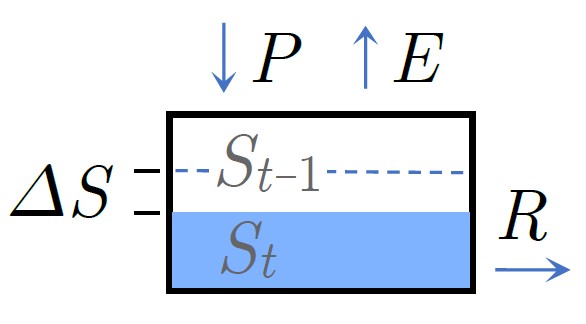
For large-scale hydrologic investigations, it is necessary to zoom out and to simplify, ignoring many minor fluxes of water. A simplified conceptual model of the water cycle includes three fluxes plus the change in storage, as shown in Figure 1.3. It fully describes the fluxes into and out of a watershed (or drainage basin). What is exciting is that three out of four of these components can now be measured by remote sensing. Further, the components of the water cycle can be described with simple equations or water budgets, described next.
A water budget is the application of the law of conservation of mass in hydrology.1 A simplified water budget for a watershed or river basin includes the four main WC components: precipitation, P, evapotranspiration E, total water storage change (TWSC in the text and ΔS in equations), and runoff, R. By conservation of mass, the water budget can be stated:
\[\ P - E - \Delta S - R = 0\]
According to scientists at the U.S. Geological Survey, “water budgets are tools that water users and managers use to quantify the hydrologic cycle. A water budget is an accounting of the rates of water movement and the change in water storage in all or parts of the atmosphere, land surface, and subsurface” (Healy et al. 2007, p. 6). An advantage of the water-budget equation is that it is simple, universal, and relies on few assumptions about the mechanisms of water movement and storage.
The water budget equation can be applied in principle over any area, or accounting unit, from 1 m² experimental plot, to a 7 million km² river basin.2 Watersheds, or river basins, make convenient accounting units. Scienists and engineers often use the water budget equation over regions other than watersheds. To use Equation 1.1 over an arbitrary geographic area, such as a grid cell, one must assume that lateral inflows are small enough to be ignored. While this is a common assumption in practice, it may not hold at all spatial and temporal scales. In a watershed, we can typically assume that there is no lateral inflow. (This is a strong assumption, and may not hold where there is groundwater flow across the basin boundary, or man-made water diversions by canal or pipeline.)
Both P and E are regularly estimated (directly or indirectly) by remote sensing. Where surface flow is confined to a river channel, outflow R, is provided by observations of river discharge. While ΔS is not a flux (the flow of matter across a boundary), it is expressed in the same units of volume per time. Throughout this thesis, I refer to these three fluxes (P, E, and R), along with total water storage change (ΔS) as water cycle components, or WC components.
Overall, this research is a form of water budget analysis, conducted at a large scale and using large amounts of remote sensing data.
Kampf et al. (2020) offer a critique of the water budget method. Practitioners ignore certain fluxes into and out of river where data are unavailable. But these are not always negligible. Examples include groundwater flow or man-made interbasin transfers. According to the authors, “such simplifying assumptions lead to missed opportunities for discovering where these unknowns in the water balance are important controls on streamflow.” The authors advocate for expanding watershed monitoring networks to include previously unmonitored fluxes to better understand “how water moves through watersheds and between the surface and subsurface at multiple spatial and temporal scales.”
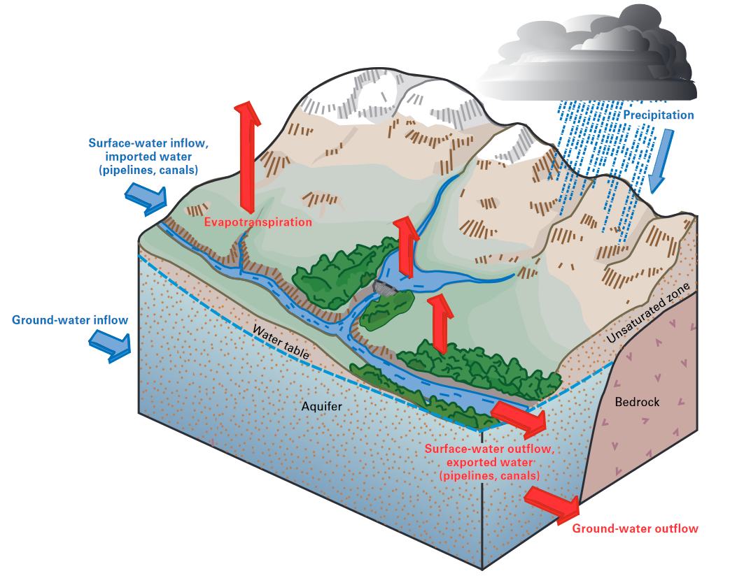
Y. Liu et al. (2020) discuss the limitations of focusing solely on surface watershed boundaries. They identify two main factors that make “effective catchment areas” differ from those defined by surface topography. The first is inter-catchment groundwater flow – that is, the movement of water into and out of the region. Subsurface flow, such as that shown in Figure 1.4, is hard to measure. In most areas, groundwater flow patterns are unknown. Yet, there is evidence that subsurface flow can be a significant contributor to the water budget in some locations (Healy et al. 2007). In practice, what we know about groundwater movement is extrapolated from modeling studies and observations at a limited number of observation wells, and estimates of groundwater fluxes have higher uncertainty than river discharge.
The second limitation of surface watershed boundaries identified by Y. Liu et al. (2020) is “limited connectivity within the catchment.” This refers to portions of the surface watershed where water does not flow toward the outlet (i.e.: there are small endorheic basins or disconnected areas inside the watershed). (For a description of how I chose to handle this issue see Section 3.1.1.)
A recent paper by Frame et al. (2023) questions the conventional wisdom of enforcing water budgets within the context of rainfall-runoff modeling. This strikes me as a radical proposal that is certain to generate controversy. The authors state that “it might not be beneficial” for hydrologic models to enforce the conservation of water mass, arguing that it prevents hydrologic models from making accurate predictions due to errors in input (precipitation) and target (streamflow) data. They conjecture that this is a reason that machine learning models (which are not required to enforce closure) often out-perform catchment-scale models in terms of predicting river discharge.
Remote sensing refers to any data collection from a distance, and includes medical imaging, radar, seismometers, etc. In this thesis, remote sensing refers to earth observation (EO) by satellites. The technology has interested hydrologists and water managers since the beginning of the satellite era. Lettenmaier et al. (2015) provides an excellent overview of developments. Some of the first satellite imagery was used to estimate snow cover in mountainous regions in 1968.
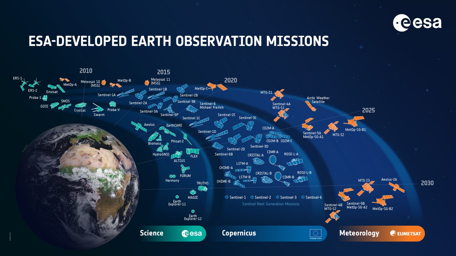
Satellites have become increasingly sophisticated in terms of the resolution of sensors and the number of bandwidths observed. Dozens of satellites are now dedicated to observation of the water cycle. Figure 1.5 begins to give an idea of the scale of the Earth Observation enterprise. A recent inventory stated that of 1,460 active satellites in orbit, 26% of these are dedicated to Earth Observation, and are operated by governments, the military, and commercial enterprises. The importance of these missions is highly recognized. Agencies begin planning for new satellite missions, and replacement satellites decades in advance, in order to provide continuous coverage and to maximize the quality of science and return on investment. The “concept-to-launch” timeline is now on the order of two decades (McCabe et al. 2017).
Satellite observations have many advantages over ground-based or in situ measurements. They offer broader spatial coverage, filling in the gaps between sparse ground stations. In remote locations or less-developed countries, remote sensing may be all that is available. Certain datasets have been published for decades, and their use is widespread, with important applications in flood forecasting, agriculture, water supply, climate modeling, and more (Lettenmaier et al. 2015). In the following sections, I give a brief overview of how satellites monitor the major components of the water cycle.
Precipitation refers to the downward flux of water from the atmosphere to the land surface. It includes rainfall and snow, and other forms of icy or frozen water like sleet and hail. Dew and fog drip are sometimes classified as precipitation (Healy et al. 2007, 36).The earliest precipitation measurements in the 1980s were based on infrared measurements of cloud-top temperatures, which are correlated with precipitation rate, oftentimes combined with measurements in the visible spectrum.
Precipitation has been described as highly fractal, as it can vary a great deal in space and time. As such, low-earth orbiting (LEO) satellites are at a disadvantage. Even with a constellation of satellites, there are usually gaps of several hours where no observations are available. Therefore, it has become common for data providers to supplement microwave data from LEO satellites with geostationary infrared satellites (Adler et al. 2018). While these observations are less accurate and have a lower resolution, they seamlessly cover much larger areas without interruption.
Each type of sensor has its advantages and disadvantages. Microwave sensors can detect emissions and lower-atmosphere scattering from rain, snow, and ice; infrared sensors measure precipitation indirectly observing cloud-top temperature and cloud height (J. Chen et al. 2020). Until 1997, retrievals relied on passive microwave observations (i.e. they measure naturally occurring microwave radiation emitted or reflected from the Earth’s surface and atmosphere). The Tropical Rainfall Measuring Mission (TRMM) was the first to include active radar, which generates microwave signals that are transmitted toward Earth and are reflected or scattered. Active microwave sensors have proven so effective that they were included in subsequent missions like CloudSat in 2006 and the Global Precipitation Measurement (GPM) mission in 2014 (Kubota et al. 2020).
Certain EO datasets of precipitation incorporate station observations (Huffman et al. 1997, e.g., GPCP). Other datasets include model output. For example, one dataset I use in this analysis, the Multi-Source Weighted-Ensemble Precipitation (MSWEP), is not a pure remote sensing product but rather an “optimal merging” of gage observations, satellite observations, and reanalysis model output (Beck et al. 2019). A good overview of the current state of the precipitation observing system, challenges, and future directions is given by Levizzani and Cattani (2019).
EO precipitation datasets have been published since the 1980s, and are calibrated to an extensive network of rain gages across the globe. As a result, their errors and uncertainties are fairly well understood and well documented, at least over regions where station density is high (Lo Conti et al. 2014; Beck et al. 2020). Biemans et al. (2009) analyzed the uncertainty in precipitation datasets, comparing seven global gridded precipitation datasets. They found that the representation of seasonality is similar in all datasets, but estimates in mean annual precipitation vary widely, particularly in mountainous regions, the arctic, and over small basins. The average precipitation uncertainty (measured by distance from the ensemble mean) over river basins was estimated to be around 30%, with variations observed between basins. The authors further analyzed the effect of this uncertainty on basin runoff. They did this by applying the seven different datasets to force the uncalibrated dynamic global vegetation and hydrology model Lund-Potsdam-Jena Managed Land over 294 river basins worldwide. Unsurprisingly, there was considerable variance in model predictions of mean annual and seasonal discharge as a result of the different forcings. The authors conclude that it is important to consider precipitation uncertainty in water resources assessments, validation, and calibration of hydrological models. As I will explain further in Chapter 3, the statistical methods used in this research rely strongly on uncertainty estimates to optimally merge different datasets.
Evaporation refers to the conversion of liquid water to water vapor. Transpiration is the loss of water vapor by plants via their stomata, the openings in leaves by which gases are exchanged. Transpiration is responsible for moving water from the soil into the atmosphere through plant growth and respiration. Because it is difficult to measure these two fluxes independently over land, they are often combined into the single term evapotranspiration. Thus, in the hydrological sciences, evapotranspiration refers to the upward flux of water vapor from land and water surfaces to the atmosphere.
On average, evapotranspiration is the second-largest water-budget component after precipitation. It is an important driver of the global climate, responsible for the exchange of water and energy from the land and sea surface to the atmosphere. It has been estimated that as a global average, evapotranspiration is about 60% to 75% of precipitation (Shiklomanov 2009).
Evapotranspiration cannot be measured directly via remote sensing. Hydrologists have created a number of climatological methods for estimating evapotranspiration, using inputs such as daily temperature, relative humidity, or solar radiation. These methods vary from purely empirical to those with a more explicit grounding in theory. Examples of such methods include Thornthwaite, Jensen-Haise, Hamon, Penman-Monteith, and Priestley-Taylor (Shuttleworth 1993).
Remote sensing data can provide the inputs to these relations, and satellite data on vegetation can help estimate the seasonal dynamics and relative magnitudes of evapotranspiration (Fisher et al. 2017). EO datasets of evapotranspiration have become more reliable and are widely used in science and water management, including water balance studies to crop performance monitoring (Mu, Zhao, and Running 2011). Yet, compared to precipitation stations, there are far fewer ground-based measurements of evapotranspiration (Fisher, Tu, and Baldocchi 2008; Paca et al. 2019). It has also been shown that different algorithms yield substantially different outputs (M. Cao et al. 2021). Both of these factors (divergent algorithms and sparse ground stations) contribute to higher uncertainties in evapotranspiration than for other water cycle components.
The Gravity Recovery and Climate Experiment (GRACE) is an innovative joint mission of NASA and the German Aerospace Center (DLR). The first pair of GRACE satellites were in operation from 2002 to 2017, and a follow-on mission began in 2018. GRACE collects detailed observations of Earth’s gravity field anomalies. Based on these anomalies, scientists are able to model how mass is distributed around the planet and how it varies over time (NASA Jet Propulsion Laboratory 2018).
Most short-term changes in the Earth’s gravity field are due to the movement of water on land and underground (Tapley et al. 2004). The gravimetric methods employed by GRACE have a solid basis in physics, yet researchers have not found an effective way to ground truth observations (Kusche et al. 2009; Reager et al. 2015). Furthermore, GRACE observations have a coarser spatial resolution than many EO data products. GRACE Level 3 data (estimates of liquid water equivalent) have been spatially filtered to remove random errors and systematic errors (F. W. Landerer and Swenson 2012). The current mascon-based solutions improve upon the older spherical harmonic solutions, eliminating the north-south striping that plagued earlier releases (Bridget R. Scanlon et al. 2016). While the datasets have a relatively high 0.25° resolution, fine scale detail (i.e. values in a single pixel) are not likely to be meaningful, and data are more accurate when averaged over larger regions (Tapley et al. 2004).
GRACE data have been used in groundbreaking studies to analyze the terrestrial water budget, drought, climate change, and water management. GRACE data have been assimilated into land surface models (Zaitchik, Rodell, and Reichle 2008; Kumar et al. 2016) and have contributed to better prediction of groundwater availability and drought. GRACE allows researchers to document water stress and groundwater declines even in regions where data from monitoring wells are not available (Konikow 2013; Richey et al. 2015; Zaki et al. 2019). Besides these examples, researchers have used GRACE data for many other applications in terrestrial hydrology – for a more complete overview see Jiang et al. (2014). Most importantly for this research, GRACE has made it possible to more completely monitor the water cycle, making it possible to perform water budget analyses. I describe over a dozen such studies in the literature review below.
Historically, hydrologic investigations were conducted by engineers for practical applications such as estimating reservoir yield or flood flows. In the last several decades, hydrologists have been increasingly interested in describing the movement of water at continental and global scales (Eagleson 1994). Large-scale hydrology is concerned with exploring “spatial scales greater than a single river basin all the way up to the entire planet” (Cloke and Hannah 2011). The sub-discipline of large-sample hydrology (LSH) often uses remote sensing data to collect data and inputs over large sets of river basins. LSH studies have made important contributions in extreme events, modeling, human impacts on hydrology, and climate change assessments (Addor et al. 2020).
Yet, the field of large-scale hydrology is not without its detractors. Kauffeldt et al. (2013) discuss the limitations of the large-scale approach to hydrology, describing some of the commonly used data and methods as “disinformative.” Among the problems identified by the authors are: (1) difficulty in accurately delineating river basin boundaries, (2) inconsistency in precipitation and evapotranspiration data, and inability to close the water balance, (3) modeled evapotranspiration that frequently exceeds physically realistic limits, and (4) basins where average runoff exceeds precipitation (not expected under natural conditions). Nevertheless, large-scales studies have made important contributions in our understanding of continental-scale water dynamics, regional water availability, and climate change impacts. Kauffeldt et al. (2013) stress the importance of screening datasets before modeling to eliminate biased datasets. This, they state, will increase confidence in the validity of model output and the chances of drawing robust conclusions from model simulations. By contrast, the philosophy behind this research is different. Rather than screening out bad datasets, or looking for the best combination, we use methods from statistics and optimization to perform data fusion. This is based on the idea that no dataset is perfect, and each can contribute valuable information.
The main goal in this thesis is to reconcile remote sensing data to “close the water cycle” or “balance the water budget.” I use both terms interchangeably, and they should be understood as referring to the same concept: reducing or eliminating the water cycle imbalance, \(I = P - E - \Delta S - R\).
Many authors have affirmed the difficulty of balancing the water budget with observations of hydrologic fluxes. Kampf et al. (2020) note that even in a highly-instrumented experimental plot less than 10 m long, the water balance is uncertain. In their view, this is because “precipitation data have biases that are not correctable, evapotranspiration is difficult to measure, and subsurface components are rarely measured.” The problem becomes even more difficult when scaled up to a large watershed with variable topography, vegetation, and aquifer properties.
The inability to close the water cycle at various spatial and temporal scales using remotely-sensed data has been widely discussed (Dorigo et al. 2021). A variety of approaches have been tested for either assessing or correcting the imbalance. I have sorted these efforts into a few broad categories, although some studies employ more than one of these methods.
Assimilation – Perhaps the most common approach focuses on assimilation of EO into hydrological models (see e.g., Yilmaz, DelSole, and Houser 2011; Yu Zhang, Pan, and Wood 2016; Wong et al. 2021). Data assimilation refers to methods for reconciling dynamical models with observations. In brief, data assimilation continuously compares new data with an existing model, and the model is updated to reflect the new conditions. For example, in the field of numerical weather forecasting, assimilation is used to update models based on observations from remote sensing, radio-sounding (balloons), aircraft, ground stations, and more. This is a large and important field with a rich literature, which however, I will not discuss further here, as my research focused on using methods other than simulation modeling.
The do-nothing approach – In one class of studies, scientists combine EO datasets without attempting to correct or reconcile them. The purpose may be to assess or document the bias or uncertainty in EO datasets. However, it is also common for scientists to assume that datasets are accurate (or at least unbiased) so that they may compute unknown water cycle components. For example, Rodell et al. (2011) estimated evapotranspiration over seven large river basins, assuming that mass is conserved and using the relation \(E = P - \Delta S - R\). (The water budget method of predicting hydrologic fluxes is discussed further in Chapter 6.)
Best combination – Some analysts compile many different EO datasets, looking for those which are most representative for their region of interest. Studies may focus on a single variable like precipitation, and compare EO data to local observations (Huang et al. 2016). Or they may combine datasets looking for the combination that results in the lowest imbalance (Wong et al. 2021). In other cases, scientists seek the combination that best predicts a single variable. Lehmann, Vishwakarma, and Bamber (2022) estimated ΔS as a function of observed and modeled P, E, and R over 189 large river basins, comparing predictions to GRACE observations. The authors looked for the best combination of input datasets that would maximize the fit between observed and predicted ΔS.
Bias-correction of individual water cycle components – Following this method, datasets are bias-corrected through comparison with in situ observations or modeled fluxes before being used in water cycle analyses. One example is provided by Schlosser and Houser (2007), who estimated global precipitation and evapotranspiration using bias-corrected reanalysis model data.
Ensemble-based methods – This approach involves averaging the water cycle components in each class. For example, multiple precipitation datasets are averaged to calculate an ensemble mean P. Examples in the literature include papers by Lorenz et al. (2014) and Lehmann, Vishwakarma, and Bamber (2022). A weighted average can be used, with weights proportional to the analyst’s confidence in a dataset. Where information on uncertainty is available, inverse-variance weighting is a popular option; however, detailed information about errors in EO datasets is rarely available (Tian and Peters-Lidard 2010).
Include energy budget constraints – For the NASA Energy and Water Cycle Study (NEWS), a pair of studies demonstrated how to explicitly couple the energy and water cycles using satellite observations over both land and oceans (L’Ecuyer et al. 2015; Rodell et al. 2015). Thomas, Dong, and Haines (2020) refined NEWS water and energy balance estimates by analyzing error covariances for ocean turbulent heat flux products (Stephens et al. 2012).
Statistical optimization – This set of methods forces water budget closure without the use of a simulation model, instead using techniques drawn from statistics and optimization. Data-driven approaches to simultaneously optimizing multiple WC components can effectively close the water cycle, redistributing errors among the various components (e.g.: Pan and Wood 2006; Aires 2014, several more references given below). This will be the focus for the remainder of this literature review, and is the approach used in this thesis.
Table 1.1 summarizes recent studies that focused on closing the water cycle with remote sensing data using statistical optimization methods. The table lists the number of datasets used in each study, and the time period (temporal domain) of the analysis. Some studies listed in Table 1.1 exclusively use remote sensing data as inputs, while others include data from models and in situ observations. The table includes a very brief description of the integration method used. Here, integration refers to the method for modifying EO datasets so that they result in closure.3
Many, but not all, of the studies listed in Table 1.1 provide estimates of the uncertainty in the optimized water cycle components, often in terms of standard deviations or 95% confidence intervals. In such cases, I briefly describe the authors’ approach to assessing uncertainty. In addition, many studies “ground truth” their results by comparing them to in situ observations. Where applicable, I include this information in the right-most column of Table 1.1.
Below, I provide some more details about some of these studies. My goal is to give a broad overview of recent work in the field, in order to put my research in context. This thesis is included in the final row of Table 1.1, and shows how this research expands upon previous work. This work includes:
Compared to previous studies, this work also introduces some methodological differences, to be described in Chapters 3 and 4. One unique aspect is my use of machine learning methods, which to the best of my knowledge, has not been used to date for closure of the water cycle using remote sensing data at the global scale.4
Table 1.1. Recent studies attempting to estimate a balanced water budget via remote sensing observations.
| Study | No. of Datasets | Study domain | Spatial scale | Temporal domain | Integration method | Method for assessing uncertainties | Data used for validating results | |||
|---|---|---|---|---|---|---|---|---|---|---|
| P | E | ΔS | R | |||||||
| Pan and Wood (2006) | 1 | 1 | 1 | 1 | One heavily instrumented experimental area in Oklahoma, USA | 0.5° grid cells | 1997 - 1999 | Constrained ensemble Kalman Filters and the VIC hydrologic model | "To evaluate the interpolation uncertainties, a “leave-one-basin-out” cross-validation procedure was performed." | in situ observed P, E, R, and soil moisture |
| Sheffield et al. (2009) | 2 | 1 | 1 | 0 | Mississippi River basin | basin | 2003 - 2006 | None. The authors purpose was to evaluate closure with EO data by estimating R = P - ET - ΔS, and evaluating the residual compared to observed discharge. | Propagated errors from inputs to predicted R via quadrature sum of errors in each component. | in situ observed R (river discharge) |
| Azarderakhsh et al. (2011) | 4 | 2 | 1 | 1 | Amazon + sub-basins | basin | 2002 - 2006 | No integration (authors searched for best combination of datasets). | - | in situ observed R |
| Sahoo et al. (2011) | 8 | 6 | 1 | 1 | Global, 10 basins | basin | 2003 - 2006 | Constrained ensemble Kalman filter | Bias and RMSE are estimated by for different satellite precipitation (P) products with respect to the non-satellite merged product over ten river basins | - |
| Pan et al. (2012) | 4 | 2 | 1 | 1 | Global, 32 basins | basin | 1984–2006 | Constrained Kalman filter | - | - |
| Munier et al. (2014) | 7 | 3 | 4 | 1 | Mississippi Basin | basin | 2002 - 2010 | Simple weighting + post filtering (OI). The OI solution is approximated for each dataset with a single linear regression model. | - | in situ observed P and E, gridded datasets of spatially interpolated observed P. |
| Lorenz et al. (2014) | 5 | 6 | 6 | 7 | Global, 96 basins | basin | 2003 - 2010 | None, looked for best combination of datasets to predict R = P - ET - ΔS | - | - |
| Lorenz et al. (2015) | 5 | 6 | 1 | 2 | Global, 29 basins | basin | 2005 - 2010 | Ensemble Kalman filter and Constrained Ensemble Kalman Filter | Range of different estimates of a variable assumed to be a proxy for the uncertainty | in situ observed R |
| Rodell et al. (2015) | 1 | 3 | 1 | 1 | Global | continents | 2002 - 2009 | "Variational framework" similar to OI, with closure at the annual time scale; a Lagrange multiplier approach is used to derive monthly fluxes | "The standard deviation across the original estimates is then taken to represent the uncertainty in the blended estimate." | Compared P, E, and R with those from 3 other published studies |
| Zhang et al. (2016) | 5 | 6 | 1 | 2 | Global | grid cells | 2004 - 2007 | Inverse variance weighting (equivalent to "simple weighting" in Aires, 2014) and Constrained Kalman Filter (CKF) method | none | R: observed discharge in 16 medium-sized basins |
| Munier and Aires (2018) | 4 | 3 | 1 | 4 | Global, 11 basins | basin, grid cell | 2002 - 2010 | Simple weighting + post filter (OI). Closure correction model, a 2- or 3-parameter regression to emulate the OI solution for each EO variable. Authors developed a 4 sets of equations for different climate zones they defined based on P, E, and vegetative cover (NDVI). | "The average of the corrected datasets (CCM with CIC) was considered as the reference to compute biases and uncertainties (standard deviation) of the corrected datasets, as well as correlation of errors." | in situ observed E |
| Zhang et al. (2018) | 4 | 8 | 3 | 4 | Global, 32 large basins | basin, grid cell | 1984 - 2010 | Constrained Kalman filter (CKF). Inputs from remote sensing, models, and observations. | "For the individual data products, their ensemble mean is taken as the best estimate for the variable, and the ensemble spread against the ensemble mean as a proxy for their uncertainty." | in situ observed R and E |
| Pellet et al. (2019a) | 4 | 3 | 4 | 2 | Mediterranean Basin, 6 sub-basins | basin | 1980 - 2009 | Simple weighting + post filter (OI). Scaling factor used to extrapolate results to sub-basin scale. | Assumed, based on standard deviation of annual predictions. | in situ observed P and E |
| Pellet et al. (2019b) | 3 | 3 | 1 | 1 | Southeast Asia, 5 basins | basin | 1980 - 2015 | Simple weighting + post filter (OI). Three-parameter regression used to extrapolate to time periods with missing data. | Comparison of the EO dataset to the OI result. Uncertainty assumed to equal the standard deviation of the residuals. | in situ observed R |
| Soltani et al. (2020) | 1 | 1 | 1 | 0 | 1 basin - Central Basin of Iran | basin | 2009 - 2016 | No integration. Calculated R = P - ET - ΔS | - | None, although authors performed a sensitivity analysis on E. |
| Pellet et al. (2021) | 4 | 3 | 5 | 1 | Amazon River Basin | basin | 2000 - 2015 | Simple weighting + post filter (OI). Regression relationship used to extrapolate to sub-basin and pixel scale. | - | ΔS from Zhang et al. (2018); R from the models ERA-Land and CAMA-Flood |
| Abolafia-Rosenzweig et al. 2021) | 5 | 3 | 4 | 3 | Global, 24 basins | basin | 2002 - 2014 | Used 3 different methods: Proportional redistribution (PR), Constrained Kalman filter (CKF), and Multiple collocation (MCL). Applied all 3 methods to each possible combination of EO datasets. | Ensemble spread as a proxy of uncertainty for water budget estimates | Compared results to the assimilation model results of Zhang et al. (2018) |
| Luo et al. (2021) | 5 | 4 | 3 | 0 | 1 basin - Tarim | basin | 2003 - 2017 | No integration (searched for best combination). Goal was to assess errors in EO datasets. | First order reliability method. Because their study basin is endorheic, there is no outflow, simplifying the water balance to 3 variables. | - |
| This study (2023) | 3 | 3 | 3 | 1 | Global, 1,698 basins | basin, grid cell | 1980 - 2019 | Inverse variance weighting (simple weighting) + Optimal Interpolation. (a) OI solution recreated with single linear regression model + parameter regionalization via spatial interpolation (kriging). (b) Neural network model to recreate the OI solution. | Uncertainty of basin-scale predictions estimated by comparing differences between model results and optimized (OI) solution; Uncertainty for P at the pixel scale estimated via comparison to gridded interpolated observations of P (CPC). | P: In situ observed P (GHCN stations); R: river discharge at gages and modeled river discharge (NLDAS and ERA-Land) E: (FluxNet); ΔS: Satellite observations (GRACE); results from previous studies (Pan and Wood, 2006; Zhang et al. 2018) |
Several of the papers in Table 1.1 use Kalman filters to close the water cycle. In brief, a Kalman filter is an efficient recursive algorithm that estimates the state of a dynamic system based on a set of noisy measurements. The process was introduced by Rudolf Kalman in the 1960s, and is now widely used in many fields, including the Earth Sciences. The ensemble Kalman filter (EnKF) expands upon this approach by using multiple model state vectors to represent the system’s state and its uncertainty. This is helpful when there are multiple sources of observations, for example from satellite remote sensing, ground radar, station observations, and ocean buoys. The EnKF method is also useful where systems have nonlinearity or high dimensionality, and is common in weather and climate models (Schillings and Stuart 2017).
Pan and Wood (2006) performed a pioneering study using the constrained ensemble Kalman filter method to estimate balanced water budget components over a heavily instrumented experimental area in Oklahoma, in the United States. The authors used EnKF and assimilation with the VIC macroscale land surface model to “optimally redistribute” water budget imbalances. Sahoo et al. (2011) merged EO datasets for P, E, and ΔS over 10 large basins, using weighted values based on their errors, to mitigate errors in the individual satellite products. The authors use the constrained ensemble Kalman filter (CenKF) method to revise water cycle components in order to satisfy the water budget closure constraint. Pan et al. (2012) used similar methods, including CenKF to merge EO datasets over 32 global river basins. In addition to remote sensing data, the authors used in situ observations, land surface model simulations, and global reanalyses.
Following a somewhat different approach, Aires (2014) introduced an integration method called optimal interpolation (OI) that draws inspiration from inversion of satellite retrievals. It is a closed-form analytical solution that imposes a WC budget closure constraint. The OI modifies each of the WC components by an amount inversely proportional to its uncertainty. Aires showed that this constraint improves the estimation of the WC components in some places and times. In a following paper Simon Munier et al. (2014) applied OI over the 3 million km² Mississippi River basin, revising satellite estimates for P, E, R, and ΔS. Optimal interpolation is at the basis of the methods used in this study, and is described more thoroughly in Section 3.8.
Multiple collocation (MCL) has also been used for solving the problem of balancing the water budget. MCL is an advancement of the triple collocation method, described well by Pan et al. (2015). Unlike methods relying on known errors in input products, MCL determines error levels based on the mutual distance (mean squared distance) among different observations, assuming their errors are uncorrelated. This a problem without a unique solution; the MCL algorithm seeks to find the best compromise in an over-constrained system. Another method for balancing water budgets is proportional redistribution (Abolafia-Rosenzweig et al. 2021). This method is perhaps the simplest of those described here, as it does not take into account uncertainties (information which is often unavailable), and simply redistributes water budget residuals to each component in proportion to its magnitude.
The techniques described above (best combination, Kalman filters, optimal interpolation, multiple collocation, and proportional redistribution) all have an important limitation. Because they require estimates of all four of the major water cycle components, they can only be applied over river basins, where estimates of river discharge can be used as a proxy for basin runoff. (For a discussion of the relationship between runoff and discharge see Section 2.5.)
Simon Munier et al. (2014) were among the first to deal with the problem of how to extend the closure analysis beyond the basin scale. What is noteworthy about their approach is that it is independent from any model. The authors created a simple linear model with auxiliary environmental variables to extend predictions to the global level at the pixel scale. In this paper, the auxiliary information was used in a fairly simple way. The authors did not us environmental data to divide basins into classes based on climate regime. (I hypothesized that predictions could be improved with a more complex model. In Section 4.4.2 I describe how environmental data are used as input variables to a neural network model.)
Later, Simon Munier and Aires (2018) applied OI over 11 large river basins, from the 620,000 km² Colorado River basin to the 4.7 million km² Amazon. OI has also been shown to work well in optimizing satellite observations of the hydrologic cycle over river basins in the Mediterranean (Pellet et al. 2018), South Asia (Pellet, Aires, Papa, et al. 2019), and the Amazon (Pellet et al. 2021).
Machine learning (ML) involves the use of computer algorithms that learn from data. In contrast, in conventional computer programs, the programmer writes explicit instructions for how to treat data. One type of machine learning algorithm, the neural network, has been the basis for some of the most exciting recent advances in artificial intelligence and computer science. Examples include large language models like ChatGPT, capable of providing detailed and coherent responses to a wide variety of questions. Another example is image generators such as Dall-E and MidJourney, which can produce extraordinary artwork based on a text “prompt” from the user. These models belong to a special class of “deep learning” models that ingest huge amounts of data during training. The large language model Chat-GPT 3.5 contains 175 billion parameters, and its successor v4 is rumored to contain 10 times more (Farseev 2023).
In the remainder of this brief literature review of machine learning in the hydrologic sciences, I describe a few interesting applications that attracted my interest for one reason or another. It is thus both brief and idiosyncratic. For a comprehensive overview of machine learning for water resources management, see a recent article by Drogkoula, Kokkinos, and Samaras (2023). The authors provide over 300 citations, covering a wide range of machine learning technologies, including many that are not discussed in this thesis. These include techniques for regression, classification, optimization, prediction, and decision support. The authors assert that the “exponential growth in data” (from remote sensing, smart devices, and social media) makes “traditional statistical mathematical approaches inadequate.”
Drogkoula and co-authors believe that ML can and will play a role in increasing human well-being through improved agriculture and better prediction of disasters like floods and droughts. With regards to the hydrologic sciences, this review cites many papers with applications, for example in hydrologic modeling and prediction, water quality analysis, data fusion, and environmental data analysis. Readers will almost certainly find something new and interesting in this review paper. If I had one critique, it is that the authors have not made an effort to rank the many ML methods they describe, in terms of their importance or use in the field.
In a similar paper, Xu and Liang (2021) summarize a great deal of recent research in machine learning and hydrology. Again, the authors cite hundreds of papers, describing research including “the detection of patterns and events such as land use change, approximation of hydrologic variables and processes such as rainfall-runoff modeling, and mining relationships among variables for identifying controlling factors.” The paper also contains a useful, if short, discussion of what the authors see as the three main challenges in applying ML in the hydrologic sciences: (1) inability to generalize results; (2) lack of physical interpretability of ML models; and (3) the small sample sizes common in hydrologic applications.
Neural networks, one type of machine learning model, have been applied in the geosciences since the 1980s for a variety of tasks in hydrology and remote sensing. For example, they have been used to classify vegetation in satellite imagery or to solve inverse radiative transfer function problems in remote sensing. Aires et al. (2001), for instance, used neural networks to estimate atmospheric water vapor, cloud liquid water, surface temperature, and emissivities over land from satellite microwave observations.
PERSIANN (Ashouri et al. 2014) is a well-known precipitation dataset that uses a neural network model to estimate rainfall intensity based on data from geostationary infrared sensors and low-earth orbiting infrared sensors. Neural networks have also been used to estimate global evapotranspiration by merging satellite and ground-based observations (Shang et al. 2021). A more detailed discussion of neural networks can be found in Section 4.4.
Another important application of machine learning methods is to estimate surface water features from satellite observations, a task which is more difficult than it sounds (Prigent et al. 2016). A recent paper by Nguyen and Aires (2023) developed a geographic “floodability index” based on topographic data. The index is defined as the probability that a pixel will be inundated compared to adjacent pixels, and is calculated at a relatively high spatial resolution of 90 meters. This index is useful for downscaling microwave-derived surface water datasets such as GIEMS, which have a coarse spatial resolution (0.25°) but have the advantage of frequent overpasses, with new estimates published monthly.
Soil moisture is another important hydrologic variable whose estimation is now frequently performed via machine learning. Soil moisture is an important variable linking the land and atmosphere and plays an important role in the carbon cycle. Soil moisture is typically estimated using both passive and active microwaves, but complications arise when applying the traditional radiative transfer model inversion approach. Kolassa et al. (2013) developed a neural network based approach to estimate soil moisture from multiple soil moisture from multi-wavelength satellite observations (active/passive microwave, infrared, and visible). The authors found that using the NN for data fusion resulted in better spatial and temporal fit to observed soil moisture. In a later application (Kolassa et al. 2016), NN models were used to merge data from two satellites (AMSR-E and ASCAT) to estimate soil moisture globally at the 0.25° scale. It appears that machine learning approaches are now widespread in the estimation of soil moisture. In late 2023, a Google Scholar search for the terms “soil moisture ” + “machine learning” + “remote sensing” returned over 36,000 results.
Machine learning methods have also been used to estimate the statistical properties of hydrologic variables such as streamflow (river discharge). Beck, Roo, and Dijk (2015) produced a set of global maps of streamflow characteristics such as the mean annual flow, the baseflow index, and flow percentiles. These statistical properties help hydrologists understand how streamflows vary in space and time and are highly useful for water supply planning and management. These quantities are well known in heavily-instrumented regions, but largely unknown over much of the Earth’s surface.
Beck, Roo, and Dijk (2015) used an NN model (a multilayer perceptron feed-forward neural network with one hidden layer containing 30 neurons) to predict streamflow characteristics based on a set of climate and physiographic characteristics (e.g. data on mean annual precipitation, temperature, topography, and soils). The results appear to be fairly good for a global study, with \(R^2\) over testing basins ranging from 0.55 to 0.93. The result is a set of maps at the 0.125° resolution, comparable to sophisticated land surface models. Further, the authors used the results to analyze “controls on streamflow,” or the factors that influence streamflow statistics. For example, there was a correlation between sand and clay composition of soils and baseflow recession. This is expected, given hydrologists conceptual understanding of watershed hydrology. These findings lend further credibility to their results, which were obtained with a relatively simple neural network model.
Recently, dozens of papers have been published which use deep neural networks to predict river discharge. A network is considered “deep” if it contains more than one hidden layer (see Section 4.4 for a description). Rainfall-runoff models have many important applications, such as forecasting droughts and floods. Recent work has shown that general-purpose deep recurrent neural networks, such as long short-term memory (LSTM) models, can produce state-of-the-art hydrologic forecasts (Nearing et al. 2021), often outperforming conventional rainfall-runoff models.
Others have investigated the feasibility of estimating river discharge using satellite remote sensing data in combination with machine learning. Dinh and Aires (2019) used a neural network model to predict discharge in large rivers in the Amazon basin using predictors derived from remote sensing data – surface water extent, water level, water volume change, and river width. The fit to gage observations was quite good (R = 0.97 for raw data, or R = 0.84 for anomalies), showing the usefulness of combining historic satellite observations and machine learning algorithms to predict hydrologic fluxes in sparsely gaged regions.
Machine learning methods have been applied to nearly every component of the water cycle, and have begun to be more widely adopted in the remote sensing community. In a recent paper by Soriot et al. (2022), machine learning methods are used to identify ice and snow cover using multiple satellites, and data collected over multiple frequencies. Snow and ice are conventionally estimated using altimetry data, observations in the visual spectra, and passive and active microwaves. An outstanding problem in the earth sciences is developing more accurate algorithms to extract geophysical products from a diverse set of measurement data. Soriot et al. (2022) combined passive and active microwave observations using a technique called Kohonen classification, a form of unsupervised machine learning. This method groups similar features in multi-dimensional datasets, preserving spatial structure. It ’self-organizes’ clusters by defining neighborhood relationships, and proved to be effective for synthesizing observations from multiple satellite instruments.
Neural networks (NNs) have also found application in water quality modeling and pollution studies. R. J. Kim, Loucks, and Stedinger (2012) used a neural network model to predict monthly watershed loading of sediment and nutrients5 over a 850 km² watershed in New York state. The authors compared the results of the NN to two conventional watershed models, Generalized Watershed Loading Functions (GWLF) and the Soil and Water Assessment Tool (SWAT), the NN models were “always essentially as accurate as those obtained with GWLF and the SWAT, and sometimes much more accurate.” The authors developed a parsimonious model, estimating the optimal number of parameters through a systematic set of trials. Their final NN model had fewer parameters (17) compared to GWLF (118) or SWAT (230).
The authors R. J. Kim, Loucks, and Stedinger (2012) obtained better results when a wider range of inputs were used to train the NN model. Initial model runs included only rainfall data, while later runs included a larger number of inputs such as temperature, wind speed, and point source discharges. Indeed, these are the same inputs that would typically be included in a conventional watershed loading model. Unlike such models, however, the NN does not make any attempt to simulate physical processes such as overland runoff, or the washoff of sediment from land surfaces. Thus, a potential critique of such a model is that it does not give any insight into sources or pathways of pollutants within the watershed. One common use of watershed models is to perform “attribution analysis,” i.e., to determine which areas or land uses are most responsible for pollutant loads.
In general, a critique of machine learning models is that they are black boxes, and while they may make accurate predictions, they do not offer any insight into the functioning of the hydrologic system (Xu and Liang 2021). This lack of interpretability limits the use of ML models in critical decision-making processes where stakeholders require transparency and explanations for the predictions. It also limits their use for scenario-based planning, a major use for hydrologic models. (For example, how does basin runoff respond to a proposed land use change?). And since machine learning models are trained on historical data, they implicitly assume that future patterns and relationships will be similar to the past. Therefore, they are unlikely to make accurate predictions in a changing environment (Hong et al. 2021).
One promising approach involves hybrid machine learning models where some knowledge of the system is coded into the network model prior to training (Moshe et al. 2020). These so-called physics-informed neural networks (Rueden et al. 2023) have shown promise in the Earth Sciences (although my experiments with them to close the water cycle were lackluster).
This study had two main objectives. The first was to optimize hydrologic EO datasets and to calculate a balanced water budgets at the river basin scale. The second objective was to train models based on these results capable of improving estimates of water cycle variables at the pixel scale. The output is a harmonized gridded dataset for the variables P, E, ΔS, and R. These data give a more complete global view of the water cycle and are useful for a variety of applications.
A third, stretch goal for the study was to test the model’s ability to indirectly estimate missing water cycle components. For example, one can estimate GRACE-like TWSC by rearranging Equation 1.1 to give \(\Delta S = P - E -R\). This allows us to fill in missing data or to estimate water storage from before GRACE was launched in 2002. Similarly, one may estimate runoff in ungaged basins, a challenge that has preoccupied hydrologists for decades (Wagener et al. 2004). Our hypothesis was that calibrated water cycle components would allow more accurate prediction of missing hydrologic variables, and better understanding of the water cycle.
My analytical approach involves optimization of satellite observations for closure of the water budget. This involves two main steps. First, I use the optimal interpolation (OI) method over a predefined set of river basins. The solution is an optimized set of water cycle components which satisfy the closure constraint.
Next, I train a set of models to emulate the OI solution, and which can be applied outside of the training basins, including at the pixel scale. I experiment with different types of models, including a simple model based on linear regression, and a more complex neural network model. The goal of the models is to calibrate EO datasets, with a goal of making them closer to the optimized version calculated by OI. This approach allows me to compare simple versus complex models for water cycle closure.
In this section, I give an overview of the organization of this thesis. This chapter, the Introduction, provided background and context for my research. The point to remember is that one cannot combine remote sensing datasets to create a balanced water budget. Solving this problem is an active field of research, but no consensus solution has emerged. Chapter 2 describes the datasets used in this research, covering all four major water cycle components: P, E, ΔS, and R. This includes data from remote sensing for the data fusion and in situ observations that will be used afterwards for evaluation. I also describe datasets describing environmental conditions: elevation, aridity, vegetative cover, and several others. These variables will be used as explanatory variables in the modeling to calibrate EO datasets.
Chapter 3 describes the methods used to create basin-scale water budgets, and details optimal interpolation (OI), a powerful analytical method for redistributing the water budget residual among water cycle components. I experiment with variants of the OI method, and conclude that using an affine error model yields the most consistent and realistic results. However, OI can only be applied over river basins where we have access to observations of all four water cycle components, including runoff. As our goal is to calibrate EO datasets at the pixel scale, another method is needed.
In Chapter 4, I describe two modeling methods that seek to recreate the OI solution, which are then used to make predictions at the pixel scale. The first method is based on fitting simple linear models, and using surface fitting methods to spatially interpolate the model parameters. The second method uses neural networks, a powerful machine learning method for estimating relationships among variables and fitting predictive models. Chapter 5 presents the results of these analyses. I analyze the modeling output in a number of ways, in order to answer certain key questions: How much do the models change the original data? How well do we close the water cycle? Is the fit to in situ observations degraded or improved?
Chapter 6 extends and further evaluates the results presented in Chapter 5. The main emphasis is on making indirect estimates of a water cycle component via the other three components. For example, one may estimate discharge in an ungaged basin with \(R = P - E - \Delta S\). There have been many studies attempting to do just this, usually with limited success. I show that using EO variables calibrated by the NN models developed here results in greatly increased predictive skill. Applications in record extension and filling missing data are discussed.
Finally, in the Conclusion, I summarize the main findings, and offer my thoughts on the significance and implications of this work. I describe which aspects of this work are novel, and help to advance research in the fields of hydrology and remote sensing. I discuss the strengths and limitations of the methods proposed here. Finally, I offer recommendations, including those for future study.
The end matter of this thesis includes a list of acronyms, followed by the complete bibliographic references. An Appendix contains additional information on remote sensing datasets in hydrology that I collected and did not use, but which may be valuable for related research.