The overall goal of the research presented in this thesis is to improve remote-sensing datasets of the terrestrial water cycle. In Chapter 1, the Introduction, I showed that the water budget cannot be balanced using remote sensing data without incurring unacceptably large errors. This leads us to conclude that one or more of the remote sensing datasets for water cycle (WC) components are biased. In this chapter, I describe analytical methods that can be used to analyze earth observation (EO) datasets, and make modifications to them to derive new estimates for components of the global water cycle.
The first section in this chapter describes the derivation of appropriate geographic boundaries for the analysis, or the delineation of river basin boundaries. First, I describe a fast method for delineating watersheds upstream of a point of interest, in this case river gages. Next, I show a method for creating “synthetic” river basins of a given size. This method allows us to create a large set of basins with global coverage using gridded terrain datasets of flow direction. This method is useful when we are working with synthetic gridded runoff data. Here, we are not constrained to using gaged sites, and may define watershed outlets wherever it is convenient. Next, I describe the conversion of vector basin boundaries to gridded basin masks. Then I detail how these masks are used to calculate spatial means of earth observations and gridded environmental data. I developed an efficient algorithm for this calculation, as it has to be repeated several million times.
Some preprocessing of EO datasets was required before they could be used in the main analyses described below. This was particularly the case for the GRACE satellite data for total water storage (TWS). I describe methods for filling gaps or missing data, and describe methods for calculating the month-over-month total water storage change (TWSC).
Next, I describe methods for combining remote sensing datasets to develop a best ensemble estimate. Following this, I describe the optimal interpolation method (and its variants) for calibrating water cycle component such that the water budget constraint is satisfied. Optimal interpolation (OI) is a simple but powerful method, but it has a serious limitation – it can only be applied over basins where runoff is available. Thus it is not generalizable; it cannot be applied to ungaged basins or to grid cells. One of the key elements of my research was investigating various modeling approaches that could “recreate” the OI solution, and which could be applied more universally, at any location and at different geographic scales. I describe two classes of models. First, a set of statistical models based on regression and geographic extrapolation with surface fitting. Second, I describe a class of machine-learning methods, namely neural network models. With any model, we are concerned with how well its predictions match observations, i.e. its goodness of fit. Therefore, I describe methods for assessing model fit that can be applied to different classes of data such as time series and gridded EO data.
River basins, or watersheds, are the most common geographic unit for analysis of the water cycle. In this thesis, I discuss analyses of the water cycle at the scale of two different geographic units: river basins and pixels. For the pixel scale analysis, I used the 0.25° and 0.5° grids described in the previous chapter. The disadvantage to studying the water balance at the pixel scale is the lack of observations of horizontal inflow or outflow. Hydrologists frequently make the simplifying assumption that there is no flow into a river basin. This means that there is no groundwater flow across basin divides, or in other words the patterns of groundwater flow in aquifers is similar to surface water flows. In other words, we assume that catchments are not “leaky” (Fan 2019). Where there is no subsurface flow across the basin boundary, we may apply the conservation of mass principle and the water budget equation. This is the key advantage of performing analyses at the scale of river basins.
A watershed is defined as the area on the Earth’s surface where water drains to a common outlet, and is determined by the topography (or elevation) of the land surface. In principle, any point on land has a watershed, that is an upstream contributing area.
To define the river basins where our water budget analysis is be conducted, my goal was fully represent the diversity of environments around the world. Basins were chosen to cover a range of climatic conditions and ecosystem types. I used the following criteria: (1) Availability and duration of river discharge measures, (2) geographic coverage – the basins should be large enough that GRACE data is reliable, and (3) geographic location.
Geographic data for watershed footprints is essential for calculating the average for WC components over the watershed. I obtained basin geodata in shapefile format from the Global Runoff Data Center (GRDC), which covered many of our gaged basins (Lehner, Verdin, and Jarvis 2008). However, some of these basin boundaries appeared to be inaccurate. I checked all basin geodata visually, overlaying the basin boundaries on topographic maps and aerial photographs. I found that some of the GRDC’s basin delineations were inaccurate. Therefore, I created a new set of boundaries for every watershed using the methods described in the next section.
Standard methods of automated (or computer-assisted) watershed delineation require large gridded (or raster) datasets that cover the entire basin to be mapped. For the best results, one should use the highest-resolution data that is available. The current state of the art for global terrain datasets is 90m resolution. However, delineating large watersheds with high resolution terrain data can be slow, requiring more than an hour for a single large watershed on a high-end desktop computer. The processing also requires more memory than is available on most desktop or laptop computers. I developed a hybrid method that is fast and accurate, which uses both vector- and raster-based data. I created a public repository to share the Python code (Heberger 2022). My method uses a vector dataset called MERIT-Basins (Lin et al. 2019, 2021), where rivers are encoded as polylines and catchment boundaries as polygons. The MERIT-Basin dataset contains 5.9 million unit catchments. The average size of a unit catchments is 45 km².
Here is a brief description of the watershed delineation method. Finding the watershed upstream of a point is a 4-step process. First, I find the river segment that corresponds to the gage, or “snap the pour point.” I created a simple algorithm that searched within a certain radius of the point to find the nearest river reach whose upstream area closely matched the reported drainage area of the gage. The process of relocating the watershed outlet point is known to be challenging (Lindsay, Rothwell, and Davies 2008; J. Xie et al. 2022), and dozens of gages required manual corrections. Second, I find the set of unit catchments that is upstream of our outlet, using a network traversal algorithm. Third, I perform a raster-based analysis to split the most downstream unit catchment, so that the watershed boundary coincides with the gage and does not include superfluous drainage area downstream of the gage.
For the detailed, raster-based calculations, I used the gridded elevation and flow-direction dataset MERIT-Hydro created by Yamazaki et al. Yamazaki et al. (2019). Finally, I merged the unit catchments in a geographic operation referred to as dissolve or unary union. The result is a single polygon that represents the drainage area upstream of the gage. I carefully reviewed the output of automated delineation routines, and made several manual corrections. I also compared the computed surface area with the reported drainage area for the gage. Where the areas differed by over 25%, I flagged these basins for more careful review.
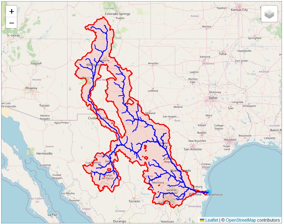
One encounters many problems when performing watershed delineation. The initial results are often incorrect, and you have to go back and make adjustments and recalculate. This was fairly easy to do with my procedure because it is very fast and the results can be visualized immediately. Some of the delineated watersheds contain internal gaps or “donut holes.” Many of these come from the source data. MERIT-Basins has many small gaps and slivers between unit catchments, often only a few pixels wide. These are obviously artifacts of the data processing, and do not appear to be meaningful. However, there are also larger donut holes inside watersheds, which represent internal sinks, out of which water cannot flow. As an example, Figure 3.1 a map of the Rio Grande watershed in the United States and Mexico, with outlet coordinates at (26.05, −97.2). Between the two main branches, the Rio Grande in the west and the Pecos River in the east, there is an endorheic basin that runs north-south for 560 km from New Mexico to Texas. Within this basin, there are several alkaline lakes or playas, a tell-tale sign that water flows in and either seeps into the ground or evaporates.
How to handle these donut holes in delineated watersheds is somewhat of an outstanding question in hydrology. These gaps represent areas that are “disconnected” and do not contribute to surface water flow at the basin outlet. How you choose to handle them may depend on the intended analysis. If we are analyzing flood flows, we perhaps ought to exclude these areas. On the other hand, if you are studying groundwater recharge within the basin, precipitation that falls in these areas may be an important contributor to the water budget.
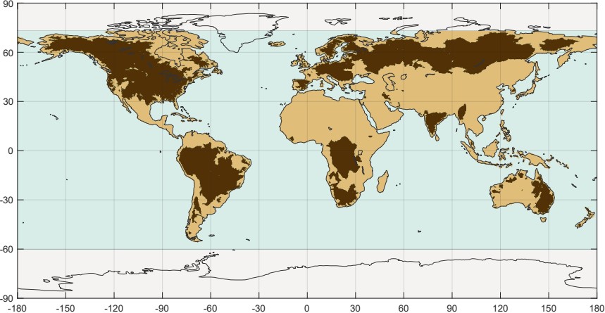
The set of gaged basins covers 47 million km², about 35% of the land surface below 73° North which is our study domain (Figure 3.2. I estimated this fraction based on a land mask from the GRACE project, clipped to the latitudes of our project area. Curiously, this layer includes Hudson Bay in Canada, and some areas of open water in the Arctic as land. This is not a concern for us, but does cause us to slightly overestimate the total land area. The total land area in our study area is 136 million km², and the area covered by our basins is approximately 47 million km². The footprint of all of our project basins is shown in Figure 3.2. On the map in Figure 3.2, the land surface in the project area is shown as tan, while the ocean and large lakes are light blue.
I created two unique identifiers for each of the 2,056 project watersheds. First, I created a set of alphanumeric codes called the basinCode. These are 10-digit strings of text, where the first two digits identify the data source, followed by an underscore, and a number. The numbers are arbitrary, but unique. Furthermore, in Matlab code, it is easier to reference data with an integer, so we created a field called basinID, where basins are identified by an integer from 1,… 2,056.
| basinCode | basinID |
|---|---|
| au_0000001 | 1 |
| au_0000002 | 2 |
| … | |
| gr_1259090 | 2056 |
I performed some exploratory data analysis of the gaged watersheds to make sure that they looked valid and correct. First, I compared the delineated watershed area to the area reported by the data provider. The GRDC reports the watershed area for many, but not all, of its gages. However, there is little metadata describing the source of this information. I noticed that it often matches the area of the shapefiles produced by Lehner (2011) and which are provided by GRDC. In other cases, I presume that the watershed area was reported by the water agency or ministry in its country of origin. I suspect that for some older gages, it was calculated by an engineer or analyst using a topographic map and a planimeter.
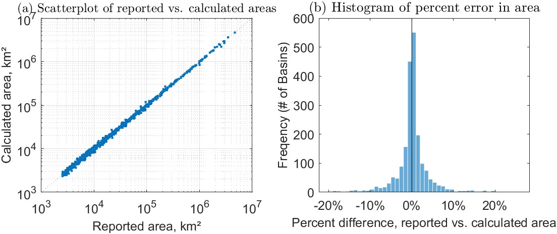
Figure 3.3(a) shows the relationship between the delineated watershed area and the reported area, in km². Note that the points are clustered very tightly around the 1:1 line, indicating the relationship is very strong and errors are relatively low (\(R^2 = 0.997\)). Figure 3.3(b) is a histogram showing the percent differences between reported and calculated watershed areas. We could call the percent difference an error; however, it is possible that the reported area is inaccurate, especially if it was estimated with older data and more approximate methods. Overall, the delineation errors here are very low compared to other large-sample hydrology studies in the literature. I attribute this to the accurate data and methods used here in addition to the “human-in-the-loop” processing method that allowed me to quickly identify and fix errors.
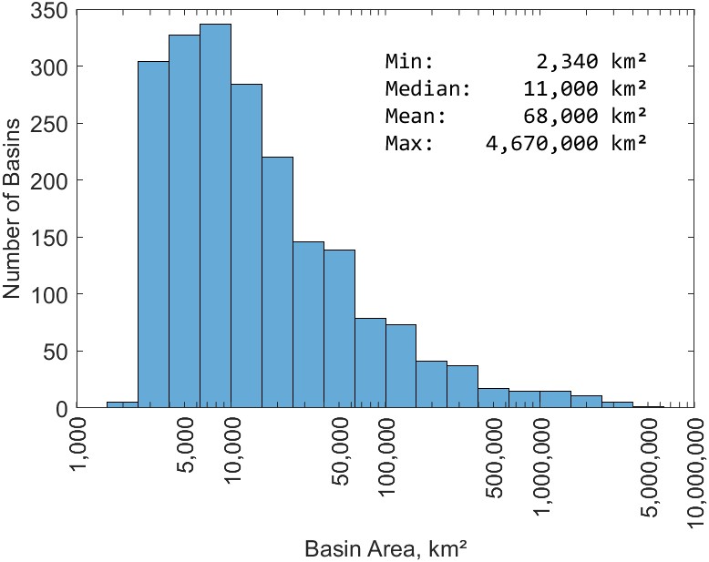
Figure 3.4 is a histogram showing the distribution of the watershed areas (in square kilometers) for the 2,056 basins selected for this study. Note that the horizontal axis is on a log scale. The distribution of basins is highly skewed, meaning that we have many small- and medium-sized basins, and there are fewer large basins. The largest basin in the study is for a gage on the Amazon River, at Obidos, Brazil, with an area of about 4.7 million km². Other large basins include the Congo River at Kinshasa (3.5 million km²), the Mississippi River at Vicksburg, Mississippi (3.0 million km²), and the Ob River at Salekhard, Russia (2.9 million km²).
In addition to the watersheds for the gaged basins, I created a second set of river basins for a set of experiments using gridded runoff data from GRUN. Here, we are not constrained by the location of river gages. Since we can calculate discharge by averaging the gridded runoff, we are free to define river basins anywhere. I refer to these synthetic basins to differentiate them from the gaged basins, which correspond to river flow gages. For the synthetic basins, their outlets do not correspond to a particular point of interest, such as a gage or an outlet. Rather, my goal was to create a collection of medium-size basins that cover much of the earth’s land surface. Note however, that the basins correspond to real drainage patterns; it is merely that the outlet locations were chosen arbitrarily (by computer code) so that the basins are of a certain size that is roughly uniform.
To create these basins, I used a gridded flow direction dataset from the creators of the Global Flood Awareness System (Harrigan et al. 2020, GloFAS). GloFAS uses the LISFLOOD hydrologic model with inputs from ERA5 meteorological reanalysis data. I obtained raster data files that contain flow direction and upstream area on a 0.1° grid.12. These data are sufficiently detailed to represent the boundaries of mid-size river basins fairly accurately, and coarse enough that we can perform calculations quickly.
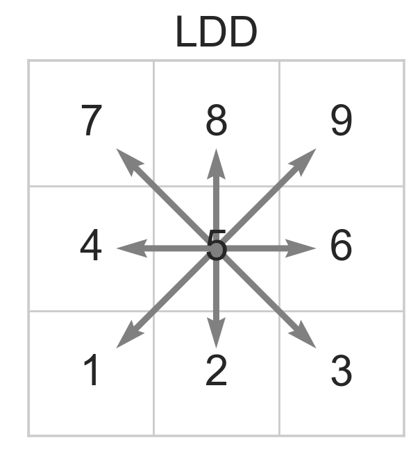
The local drainage direction (LDD) file uses 8-direction (D8) encoding, using the conventions of PC-Raster environmental modeling software (Karssenberg et al. 2010). The direction of flow is coded as an integer from 1 to 9, as shown in Figure 3.5. In this scheme, a missing or NaN (not a number) value indicates outflow to the ocean, and a value of 5 means the pixel is a sink.
I used the open source Python library pysheds (Bartos et al. 2023) to create a flow accumulation grid. This is a standard data file that is used in terrain analysis and watershed delineation. There are two types of flow accumulation grids that are commonly used for watershed delineation. In the first type, each pixel contains a value representing the number of upstream cells. In the second type, each pixel contains its upstream drainage area, for example in km². I wrote a Matlab script to find the cells where the upstream area fell within a given size range. After some experimentation, and in consultation with my advisor, I chose to find basins ranging from 20,000 to 50,000 km². This size range was selected to balance the competing desire of using large river basins versus having a large sample size.13
My routine for finding river basins required a data structure that inverts the downstream flow direction and instead reports the upstream cells. For this, I created a matrix listing the upstream neighbors of each cell. There are 6,480,000 cells (in the 3600 × 1800 grid), and each cell can have up to 8 upstream neighbors. Therefore, the upstream neighbor matrix has 6,480,000 and 8 columns. Using this information, I found the set of grid cells that defines the upstream drainage areas.
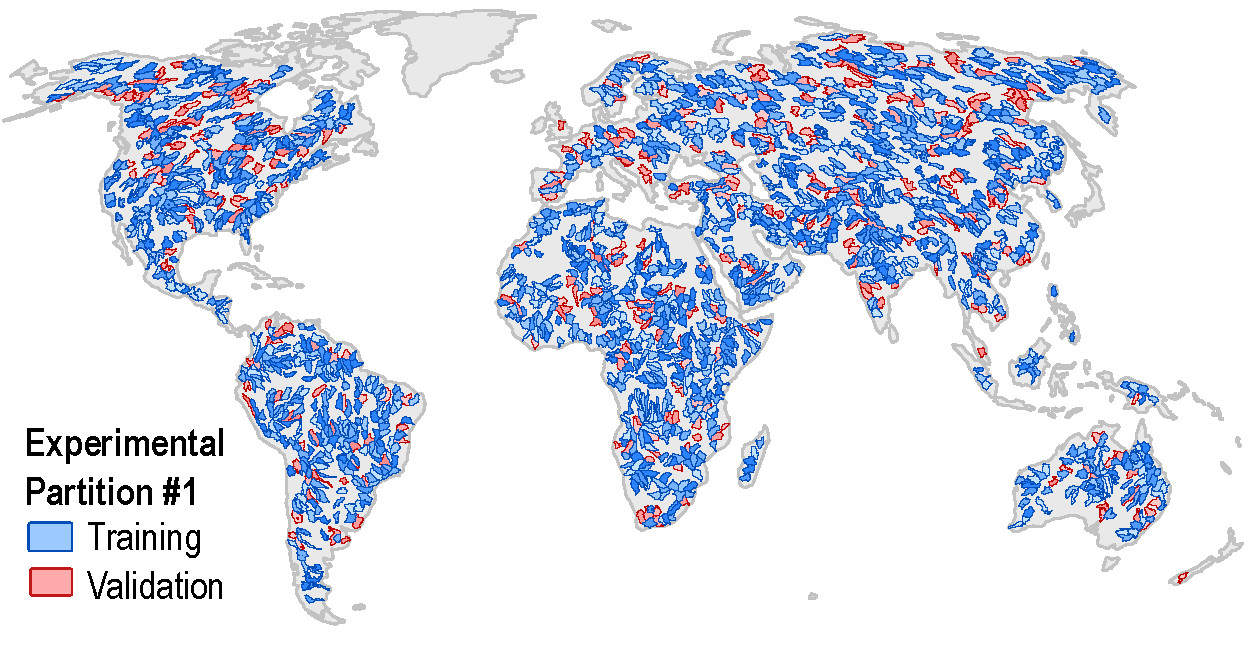
Figure 3.6 shows the 1,698 synthetic river basins. The color coding is for one of several sets of experimental partitions created for the training and validation of the neural network model, with the 80% of basins in blue for training, and 20% of basins in red for validation.14 If we compare the set of synthetic basins shown here in Figure 3.6 to the set of gages in Figure 2.8, we see that it provides much better spatial coverage. As discussed in Section 2.5.1, there are large gaps in the availability of gage data over our period of interest (2000 - 2019), especially over Africa and Asia.
As described in Chapter 2, there are many missing records in the GRACE dataset of total water storage. In this section, I describe a simple method to fill in gaps in the record based on interpolation. I only use this method where I have reasonably high confidence in the interpolated value. In cases where the estimate is highly uncertain, more detailed methods based on modeling or water budget analysis may be more suitable for reconstructing GRACE-like TWS data, and filling in missing data. For one such example of methods to fill in missing data, see Yi and Sneeuw (2021). Other studies have focused on reconstructing the GRACE signal of TWS via modeling or regression-based methods, in order to hindcast, or create data from before the GRACE satellites were launched (see e.g., Fupeng Li et al. 2021).
I calculated the month-over-month rate of change in water storage to provide the flux in mm/month. This converts the TWS anomaly to a flux equivalent, TWSC or ΔS. There are several methods for calculating the rate of change, but most researchers in this field use simple finite difference methods (see e.g., F. W. Landerer and Swenson 2012; Biancamaria et al. 2019). I chose the simple backwards finite difference method.
\[ \frac{\Delta S}{\Delta t} = \frac{S_{t} - S_{t - 1}}{t - (t - 1)} \label{eq:delta_s} \]
Results from more complex methods such as fitting a cubic spline or using an “equivalent smoothing filter” (Landerer, Dickey, and Güntner 2010, see e.g.,) were comparable to those obtained with the simpler methods but often resulted in more missing observations, therefore I chose used the simple method in Equation \ref{eq:delta_s}.
The amount of missing data in the water storage time series threatened to limit our analyses. Therefore, we used methods from time series analysis regularly used by earth scientists to fill in missing observations. The GRACE water storage observations begin in April 2002. Following a few missing months (gaps) in the beginning, and then there is a 6-year record with no gaps from 2004 to 2010. However, as the GRACE satellites aged, they were plagued by various issues such as failing batteries, and the satellites were powered down intermittently, resulting in intermittent 2-month-long gaps occurring regularly. The first satellite mission ended in 2017, and there is a 11-month gap until the follow-on mission was launched and began operating in 2018. We focused on filling the shorter 1-3 month gaps, and made no attempt at filling the 11-month gap between the two missions.
In the earth sciences, it is common for a dataset to be missing observations, for a variety of reasons, such as instrument failure, calibration problems. Instead of discarding these incomplete records, a commonly applied approach is to perform imputation, which involves filling in the missing values. I used standard time series analysis methods to fill in some missing observations via interpolation. In order to limit the uncertainty of interpolated observations, we did not allow the routine to fill gaps longer than 3 months.15 Further, we did not fill in missing observations where there is a change in slope in the time series before and after the gap. Because the missing observation would represent either a peak or a trough, attempting to impute the missing value would be highly uncertain. As a result of the missing data, maps of ΔS for interpolated months appear patchy and incomplete. That is because I only filled in missing data with interpolation where the estimate has high confidence, as described above.
Certain datasets are published in a higher resolution than that of our analyses. In such cases, I used upscaling methods to create a lower-resolution versions of the high-resolution datasets. For example, I upscaled vegetation data (EVI and NDVI) from 0.05° to 0.25° resolution. There are several different methods available for doing this, with tools available in GDAL (gdalwarp), and using Matlab (interp2 or imresize are two options).
For upscaling, I used a “correspondence matrix.” This matrix contains a complete mixing of how pixels in the fine grid correspond to pixels in the coarse grid. This method is fast and gives“pixel-perfect” results. The correspondence matrix method only works when the high resolution is evenly divisible by the coarse resolution, for example going from 0.05° to 0.25° resolution. In such cases, the smaller pixels are fully contained within the larger pixels with no overlapping of edges. In this example, the detailed dataset is exactly 5 times the resolution of our target result. So each large pixel contains exactly 25 of the smaller pixels in the source dataset. We can simply take their arithmetic mean of 25 pixels to calculate the average in the large pixel. This approach (taking the average of overlapping grid cells) does not incorporate any smoothing or blurring. By contrast, these are features of some rescaling algorithms, which consider the values in neighboring cells when rescaling.
The algorithm I used takes missing values into account. Missing data are quite common, due to cloud cover, sunglint, or other factors. Because the vegetation datasets only cover land surfaces, there are no data over oceans and lakes. We should not allow a few missing values to prevent us from calculating the average over the larger pixel. In my experiments, doing so results in a large amount of missing data, especially near the coasts. Therefore, I used a compromise algorithm with the following rule. If a majority of pixels are available (do not contain the missing data flag), we calculate the average based on available data. For example, when we are upscaling from 0.05° to 0.25°, we must have valid data in 13 or more of the 25 small pixels.
What about the case where the lower resolution is not evenly divisible by the higher resolution? For example, suppose we are upscaling a dataset from 0.1° to 0.25° resolution. In this case, I used a two-step procedure. First, we rescale the high-resolution raster dataset using Matlab’s imresize function. This is part of Matlab’s Image Processing toolbox, and is originally intended for processing image data, but it works equally well on any sort of regular two-dimensional grid. We can instruct Matlab to use a “box-shaped kernel” over which to average the high-resolution data. We can also instruct it to omit NaN values (“not a number,” a stand-in for missing data in a pixel). The risk here is we may end up with some pixels in the resulting lower-resolution output that are based on very few valid observations. At the upper limit, the result could be based on a single small pixel. Since such results are not very robust, I performed a separate calculation to count the number of pixels with missing data. If the percent of missing pixels is below a threshold, we declare that the calculation is low-quality, and discard it. I used the cutoff of 50%, meaning that if more than 50% of pixels are missing, the result is discarded. This allowed a good compromise between obtaining a complete coverage and a robust calculation of the mean. The choice of the 50% threshold was arbitrary. In practice, varying the threshold between 25% and 75% did not have a major impact on the results.
For each basin, I calculated the average P, E, ΔS, and R based on the gridded EO data products. I followed similar methods to those described by Kauffeldt et al. (2013). In brief, basin polygons are intersected with climate-data grid cells to calculate the fraction of precipitation (or other variable) that each cell contributes to the basin. This method relies on the assumption that there is no sub-grid variability, i.e. precipitation is assumed to be evenly distributed over each grid cell.
In geographic science, there are “zonal statistics” methods for calculating the statistics of gridded or raster datasets where they overlay or intersect a vector polygon. However, it was more efficient for me to use matrix math and perform the calculations in Matlab. To calculate the spatial weighted mean, I converted each basin polygon to a grid mask, where each pixel is a floating-point number representing the fraction of the pixel’s area from 0 to 1 that is inside the basin. Because the surface area of pixels varies by latitude, I also use the pixel’s area in our calculation via the Climate Data Toolbox for Matlab (Greene et al. 2019). The same routine was also used on all other gridded data products, such as the aridity index, vegetation indices, and elevation.
In this section, I describe how I calculated the average of gridded environmental data over watersheds. This is a common task in the environmental sciences, but it is worth describing for two reasons. First, this research required calculating basin means tens of thousands of times, so an efficient method is required. The first large-scale experiment described here used 2,056 basins, 10 variables, and 240 months; thus I repeated this calculation around 4.9 million times (actually somewhat less due to missing data). Second, this calculation is not always done correctly, even by experienced scientists. Witness a recent retraction in the prestigious journal Nature. The authors incorrectly calculated precipitation over river basins. The authors incorrectly used arithmetic averaging to calculate the mean, “instead of calculating a spatially weighted mean to account for the changing grid box size with latitude” (Marcus 2022). As a result, the results were biased and the conclusions not supported, forcing the authors to retract the paper.
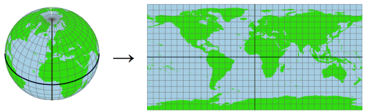
When working with data on a regular rectangular grid, it is important to understand that the area of the grid cells varies as a function of latitude. Figure 3.7 shows how the grid cells on the three-dimensional sphere of the Earth16 are stretched and distorted when they are represented in two dimensions. Figure 3.7 shows 10° × 10° grid cells for clarity, rather than the smaller 0.25° or 0.5° grid cells of our EO data.
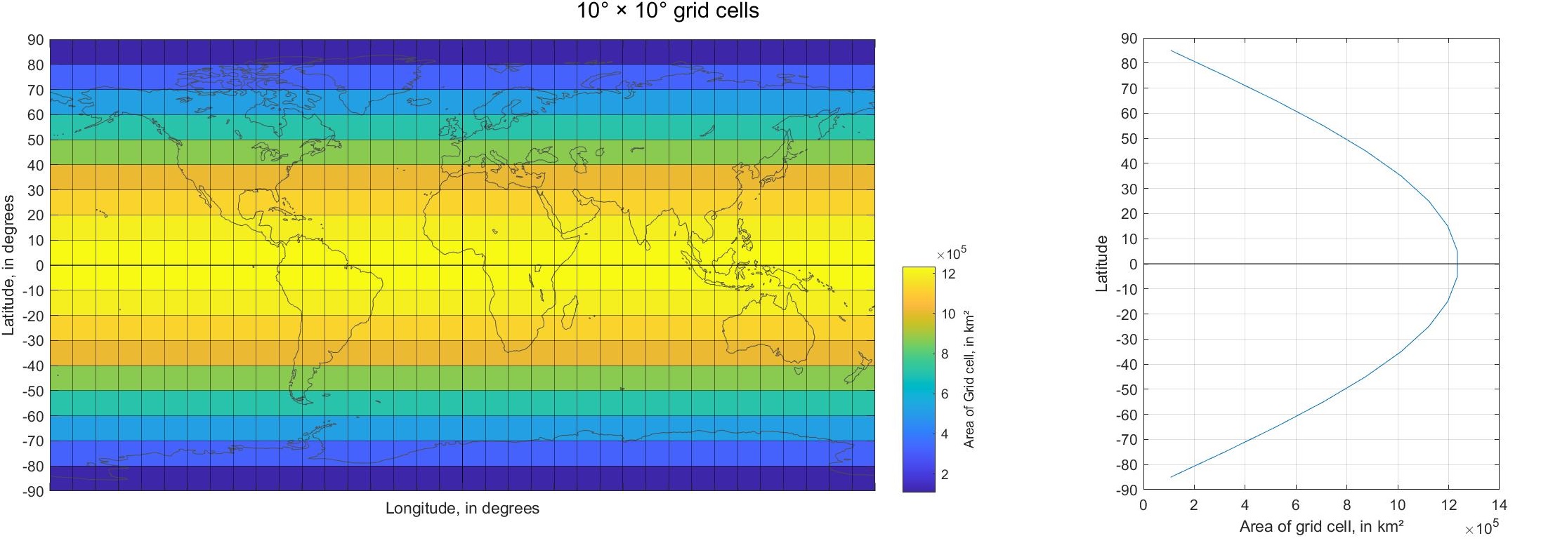
The surface area of grid cells is the maximum at the equator, and decreases as we move north or south, away from the equator and toward the poles. Figure 3.8 shows how the surface area of grid cells varies as a function of latitude. Again, this figure shows a 10° grid to demonstrate the concept.
To calculate the basin mean of an EO variable, we average the values of the pixels over the basin. However, because the pixels are of irregular size, we take a weighted average, where each pixel is weighted based on its surface area. Calculating the basin mean is a type of “zonal statistics,” commonly calculated in geographic science. It is complicated somewhat by the fact that we are overlaying two distinct and incompatible data types. Basins are represented by vector polygons, and the earth observation datasets are grids or rasters. We can speed up the calculation of the spatial mean by converting the basin to a ‘mask’ in grid format. In this way, we can use fast and efficient matrix math to calculate spatially-weighted basin means.
I created two sets of masks for the basins:
In Geographic Information System (GIS) software, converting a vector feature to a grid is called rasterization. GDAL is a widely used open-source library for performing many geoprocessing operations. I used the GDAL function rasterize to convert watershed polygons to a grid.
The initial results of the vector-to-grid conversion were unsatisfactory zoomed in to the pixel level. Since we are interested in some watersheds that cover only 8 pixels, we want to have the results as realistic as possible. The way that GDAL’s rasterize algorithm determines whether a pixel is inside of a polygon is by looking at the centroid of the pixel. So you can encounter a situation where a polygon covers over half of pixel, but the pixel is not included in the raster output, because it was incorrectly classified as non-overlapping. Such considerations may be trivial when dealing with large features covering an area of thousands of pixels. But because some of our watersheds only cover about 8 pixels, I wished to avoid such rasterization errors. In other words, I was looking for “pixel-perfect” results. So I created a custom rasterization procedure using Python for QGIS. The following is an overview of the steps in the process.
There is a single input to my pixel-perfect rasterization algorithm: a vector polygon in shapefile format, representing the basin or watershed. Figure 3.9(a) shows an example of a watershed of GRDC gage 1159511 on South Africa’s Vals River at Groodtraai. The polygon has an area of 7,801 km². The algorithm for calculating a higher-precision floating-point raster involves rasterizing at a 5x greater resolution, shown in Figure 3.9(b). This intermediate raster file has 25 times more pixels. In this example, to create a 0.25° raster mask, we first create a raster mask at 0.05°. In this intermediate file, cells have a value of 0 or 1. A single grid cell is covered by a 5 x 5 set of grid cells in the higher-resolution dataset. Then I calculate the sum of the small cells that are in each large cell. The result is the fraction of the large cell that overlaps the basin polygon.
The rasterization routine produces the outputs shown in Figure 3.9(c) and (d). The version on the left in (c) is a floating point raster, where the value in each cell represents the fraction of that pixel that is in the basin. The map on the bottom right (d) shows the Boolean (0/1 or true/false) version of the basin raster. The floating-point raster is able to preserve more information about the river basin’s geographic coverage, which allows us to better estimate the WC components over the basin from gridded EO data.
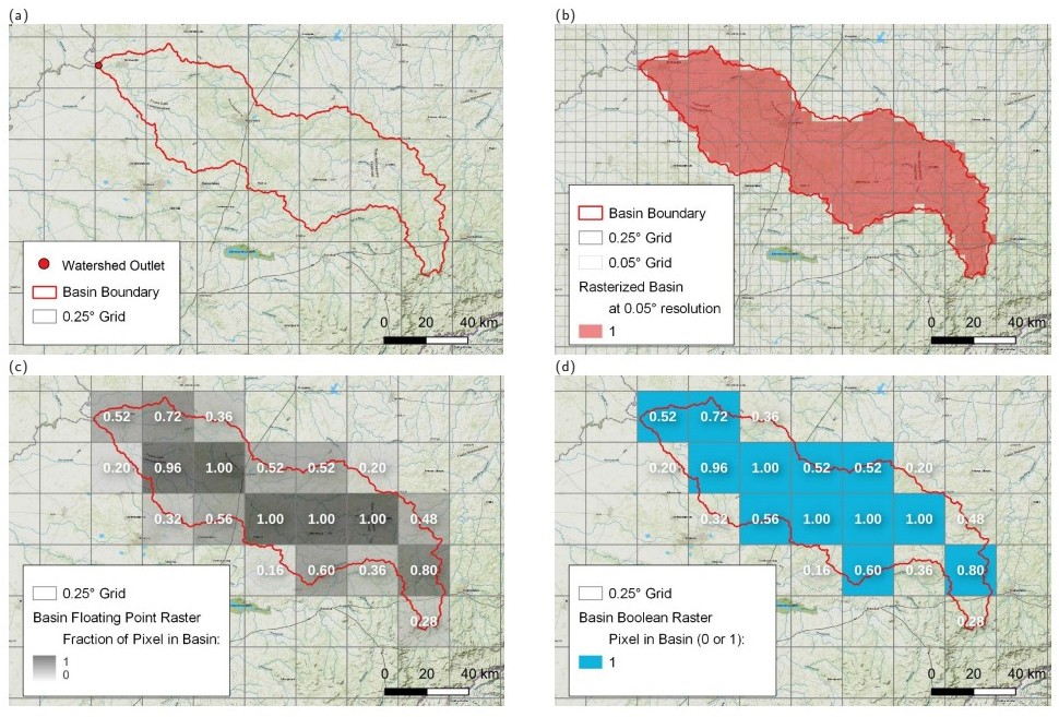
Table 3.1 summarizes the rasterized basin mask for our example basin, the Vals River watershed shown in Figure 3.9. Note that the Boolean mask contains fewer total pixels, but has a larger surface area. The Float mask contains more pixels in total, but most of the pixels have a value less than one, indicating that it is only partially contained in the basin. Overall, its weighted area (7,909 km² is lower, and much closer to the area of the vector polygon (7,901 km²), a difference of only 0.1%.
Table 3.1: Statistics for basin masks.
| # Pixels | Mask Area (km²) | P (mm/month) | |
|---|---|---|---|
| Vector | 7,801 | ||
| Boolean | 12 | 8,213 | 82.0 |
| Float | 20 | 7,909 | 78.6 |
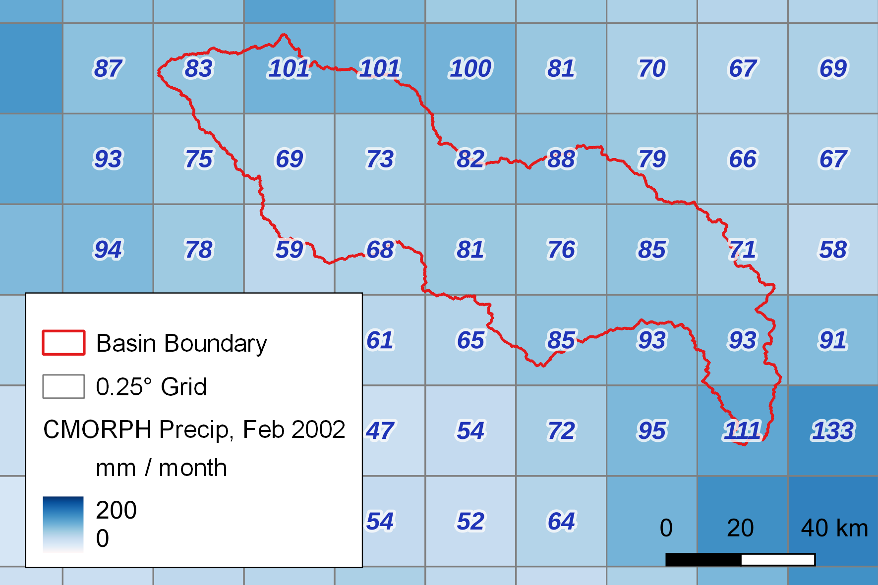
As an example, I calculated the basin mean precipitation over the Vals River basin for February 2001, using CMORPH data, shown in Figure 3.10.
In order to calculate the spatially-weighted area, we first need the area for grid cells. I calculated A, the area for grid cells, using the function cdtarea in the Matlab Climate Data Toolbox (Greene et al. 2019). The function returns the approximate area of cells in a latitude/longitude grid assuming an ellipsoidal Earth. This authors intend the function “to enable easy area-averaged weighting of large gridded climate datasets.” The area, A, of a grid cell is:
\[ \label{eq:grid_cell_area} \begin{aligned} dy &= dlat \cdot R \cdot \pi / 180; \\ dx &= dlon / 180 \cdot \pi \cdot R \cdot \cos(lat); \\ A &= \left| dx \cdot dy \right| \end{aligned}\]
where \(lat\) is the latitude of the center of the grid cell, \(dlat\) is the height of the grid cell, and \(dlon\) is its width, all in decimal degrees. The radius of the earth, R, is based an ellipsoid model. Because the Earth is not a perfect sphere but an oblate spheroid, R varies according to latitude, as follows:
\[\begin{aligned} R &= \sqrt{ \frac{{(a^2 \cdot \cos(lat))^2 + (b^2 \cdot \sin(lat))^2}}{{(a \cdot \cos(lat))^2 + (b \cdot \sin(lat))^2}} } \\ \mathrm{where:} \\ a &= 6,378,137 \text{ (Earth's equatorial radius, in meters)} \\ b &= 6,356,752 \text{ (Earth's polar radius, in meters)} \\ \end{aligned}\]
While it is not documented in the Climate Data Toolbox, the values A and \(b\) for the Earth’s equatorial and polar radii are from the World Geodetic System 1984 (WGS-84) reference ellipsoid, which is currently widely used for mapping and satellite navigation (NGA 2023).
The formula for calculating the spatially weighted mean of a climate variable, such as the example in Figure 3.10, is as follows:
\[\bar{P_{b}} = \frac{\displaystyle{\sum_{i=1}^{m} \sum_{j=1}^{n} B_{i,j} \,A_{i,j} \, P_{i,j}}} {\displaystyle{\sum_{i=1}^{m} \sum_{j=1}^{n} B_{i,j} \, A_{i,j}} }\]
where we are summing over all the grid rows i from 1 to \(m\), and over all columns \(j\) from 1 to \(n\), \(B\) is the Boolean basin mask, A is the grid cell area in km² from Equation \ref{eq:grid_cell_area}, and P is the precipitation in mm/month.
In principle, we can sum over all i and \(j\) (i.e., every pixel on the planet), but the calculations are faster if we restrict i and \(j\) to those which are members of the basin, i.e. where \(B = 1\). In practice, the Matlab code handles this automatically when we declare the grid mask as a sparse matrix. A sparse matrix is one where most of its elements are zero.
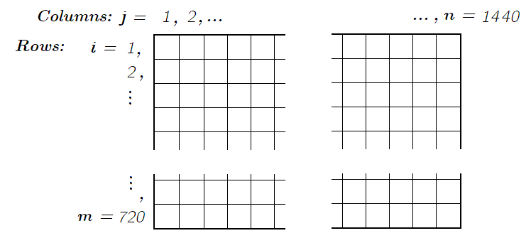
Figure 3.11 shows the grid cell indexing, or numbering scheme used throughout the project. This is worth noting clearly here as different conventions are used by different agencies and research teams. In our grid, row numbering begins at the top of the globe (the north pole, or latitude +90° N) and increases as we move down or south. Rows are numbered from 1 to 720.17 We use the variable i to refer to the row number, and the number of rows is \(m\). Columns begin at longitude −180°, a line running north to south through the Pacific Ocean beginning in the north west of the Aleutian Islands, over Russia’s Chukotka Penninsula. Columns are indexed from \(j = 1, 2, \ldots, n\).
Finally, a note about the location of the pixels on the grid. The top edge of pixel (1, 1) is at 90° latitude, and its left edge is at −180° longitude. The centroid of this pixel has latitude/longitude coordinates of (89.875, −179.875). Again, this is worth noting, as some data providers use a different convention of locating the centroid of the first column at −180. When this alternative convention is employed, an extra column of pixels is required to cover the globe. When this mapping method is used, a 0.25° global grid has 721 rows and 1441 columns. Compared to an ordinary edge-matched grid, there is a half-pixel width overlap where the eastern and western edge of the map join. These are small but important details that require careful attention of the programmer when dealing with data from multiple sources.
To calculate the area with the floating point basin mask, the formula is similar, but we multiply the terms in both the numerator and the denominator by the fraction in the basin:
\[\bar{P_{f}} = \frac{\displaystyle{\sum_{i=1}^{m} \sum_{j=1}^{n} F_{i,j} \,A_{i,j} \, P_{i,j}}} {\displaystyle{\sum_{i=1}^{m} \sum_{j=1}^{n} F_{i,j} \, A_{i,j}}}\]
where \(F\) is the floating point basin mask, and \(0 \leq F \leq 1\).
I wrote efficient Matlab code using sparse matrices to speed up the calculation. The code also vectorizes two-dimensional matrices to avoid using loops in the code, which provides the biggest boost to calculation speed. Initial code implementations for calculating basin means of EO variables (obtained from other researchers in my laboratory) took 3 to 4 seconds on a laptop computer. Because I had to repeat this calculation many thousands of times, it was important to reduce the processing time. The new, efficient version reduced this to 15 to 20 milliseconds. This cut the total processing time from hours to minutes. This function, calc_basin_mean(), is available in the code repository accompanying this thesis.
In this section, we explore the earth observation (EO) datasets that we compiled to analyze the water cycle in river basins across the globe. I attempt to quantify the water budget with uncorrected EO data and show that it results in large budget residuals at both the pixel scale and river basin scale. The EO datasets referred to here as uncorrected are far from being raw data. Data on precipitation, for example, are typically calibrated to millions of observations collected at thousands of locations. Yet, our hypothesis is that further improvements are possible by cross-calibrating using data for other water cycle components.
This analysis reveals the extent to which there is a lack of consensus in predicting water cycle components. I also show the locations where the variance among different datasets is most pronounced.
The overarching goal of this research is to optimize earth observations of the water cycle. We saw previously that it is not possible to create a balanced water budget (or “close the water cycle”) using EO datasets. In principle, the fluxes plus change in storage over any given region should sum to zero, as expressed in Equation 1.1. However, this is rarely the case, leading us to the conclusion that one or more of the data layers contains errors. Recent research in hydrology and remote sensing has focused on how to combine or merge multiple datasets to reduce these errors; for a review of the literature on this subject, see Section 1.3.1. Our hypothesis is that there is a benefit of combining multiple classes of observations. Rather than focusing on calibrating individual water cycle components (for example precipitation), we seek to optimize all four components (P, E, ΔS, and R) simultaneously.
Figure 3.12 shows the water cycle imbalance for each of the 27 possible combinations of EO variables. The variables in this analysis are listed in Table 2.1. There are 3 variables each for P, E, and ΔS, and 1 for observed R. The combinations are color-coded by the precipitation data source, which appears to have a large impact on the imbalance. Figure 3.12 also shows the simple weighted average solution as a black line, calculated as \(I_{SW} = \bar{P} - \bar{E} - \bar{\Delta S}\). We can see that the simple step of averaging multiple datasets results in an imbalance that is less biased.
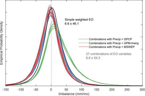
We can see from Figure 3.12 that the combinations that include precipitation from the GPM-IMERG dataset (light green lines) tend to have a higher imbalance than the other combinations, on average. The precipitation estimates are therefore more incoherent with the other water components. In addition, GPM-IMERG precipitation is higher on average than the other precipitation datasets. This can be seen in Figure 3.13, which shows the monthly mean precipitation over continental land surfaces.
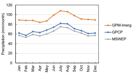
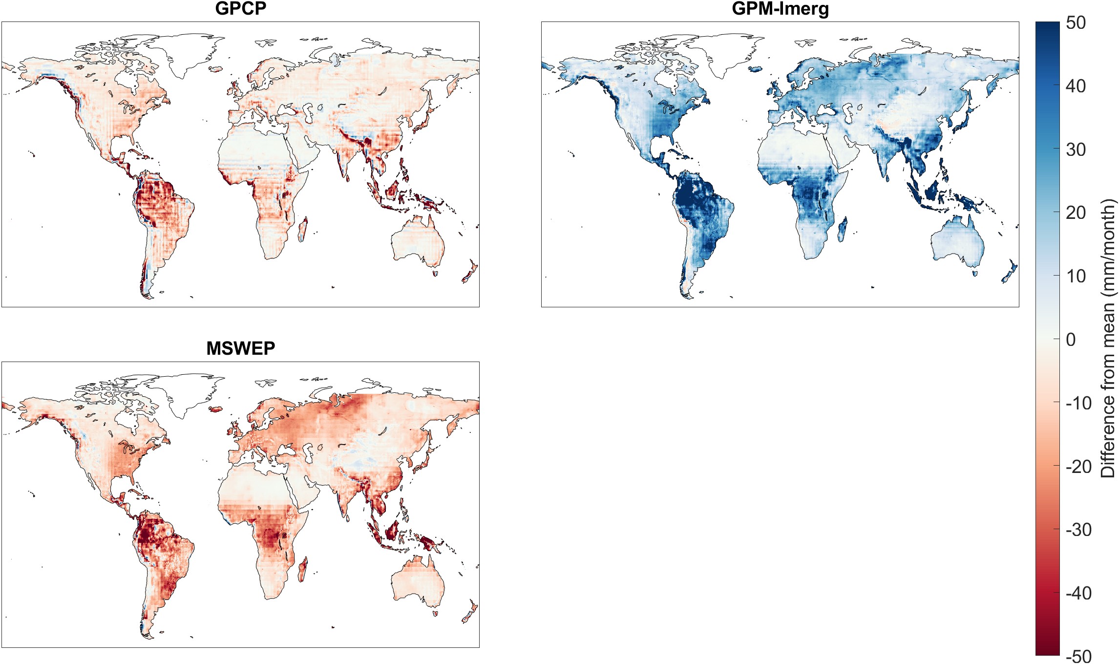
The GPM-IMERG dataset reports higher precipitation amounts, on average, across all months, compared to the GPCP and MSWEP datasets. This is illustrated in the set of maps in Figure 3.14. Each map shows the difference between average precipitation calculated in each grid cell, and the 3-member ensemble mean. Overall, GPM-IMERG reports higher precipitation across the globe as well, with the exception of the extreme west coast of South America, portions of Western North America, and around the Himalayan plateau in Asia. The differences can be quite large, up to 50 mm/month or more.
Our goal is to make adjustments to remotely sensed observations of WC components such that the water cycle is balanced and hence improved. We seek to make these adjustments in a way that is methodical, mathematically rigorous, and has a solid basis in information theory. At the heart of our method is the idea that, for values with greater error or uncertainty, we have less confidence in their correctness, and therefore we will change them more. And for variables with a lower uncertainty, we are more confident that it is close to the correct value, and we will change them less.
Remote sensing of precipitation or another hydrologic variable involves a number of sources of uncertainty, which can be broadly categorized as reducible and irreducible uncertainties. Reducible uncertainties are those that can be reduced through improved measurement techniques, data processing algorithms, or calibration/validation procedures (Njoku and Li 1999). Some sources of reducible uncertainty include errors in instrument calibration or in atmospheric correction algorithms, geolocation accuracy, and inversion algorithms. Irreducible uncertainties, on the other hand, are those that cannot be eliminated. Some sources of irreducible uncertainty are due to limitations of the instruments and sampling rate. Variables such as precipitation are highly variable in space and time, and often cannot be fully captured by remote sensing.
I follow previous studies (Aires 2014; Pellet, Aires, Munier, et al. 2019) in using Optimal Interpolation (OI) to integrate satellite-derived datasets and balance the water budget at the river basin scale. The OI method has been demonstrated and applied in several studies: over the Mississippi River Basin (Simon Munier et al. 2014), over the Mediterranean Basin (Pellet, Aires, Munier, et al. 2019), and over five large river basins in South Asia (Pellet, Aires, Papa, et al. 2019).
The overall approach is based on forcing the imbalance, I, to equal zero. The OI calculation has two basic steps. First, we calculate a weighted average for each flux based on our input data, selected from among available EO datasets. This weighted average provides our best initial estimate for P, E, ΔS, and R. Next, the water budget residual is redistributed among each of the four water budget components using a post-filter matrix. OI makes adjustments to each variable in inverse proportion to the variable’s uncertainty. This class of methods is well-known in the field of remote sensing, and their use in hydrology was introduced by Aires (2014). Such methods, well described by Rodgers (2000), are referred to as inverse methods and are widely used for remote sensing. In the following section, I introduce the mathematical notation and show how the calculations are done.
The equations below show how to redistribute the errors and balance the water budget for a single observation. In other words, we are dealing with the fluxes at one location and one time step. In this case, an observation is for a single river basin in a single month. This method does not distribute errors spatially among neighboring basins or pixels. Nor does it involve distributing errors over time, i.e. the month before or after the observation. Note that the equations and sample calculations shown here cover a single observation, with the inputs in the form of a vector. Multiple vectors are readily stacked into a matrix, and the calculations can be performed very efficiently, even with millions of observations.
We begin with the problem of combining multiple satellite estimates of WC components. As we saw in Chapter 2, there are many earth observation datasets available for hydrologic variables. Indeed, I described over a dozen precipitation datasets, each of which are freely available and widely used. What does a practitioner do when faced with so much information? There are several common approaches. First, the analyst may choose a particular dataset out of custom or preference, or because a dataset is in a format that is compatible with existing software code. Other times, an analyst will do an intercomparison analysis to find the dataset which is most representative of their study area. A common approach is to compare the gridded data to in situ observations to determine which is the most representative of the target region (see e.g., Kidd et al. 2012; Duan et al. 2016; Huang et al. 2016). Another approach is to use the different datasets as inputs to a hydrologic model, and determine which ones result in the best predictions of observed runoff (Seyyedi et al. 2015; Guo et al. 2022).
Other analysts choose an ensemble approach, and simply average multiple datasets. The ensemble philosophy is that no-single “best-estimate” exists (Abolafia-Rosenzweig et al. 2021). This approach is commonly used in assessments of climate change. There are numerous climate models, and each gives somewhat different predictions of future climate. By considering the outputs of several models, the analyst can begin to see where there is consensus, and which outcomes are more uncertain. In the hydrologic sciences, rainfall-runoff modelers often combine data on precipitation from multiple sources (for example from radar, remote sensing, and gages). Using multiple sources allows the modeler to better capture the spatial and temporal variability of rainfall within the catchment (H. Liu et al. 2021). The ensemble approach is particularly valuable for flood forecasting, where the forcing is based on meteorological models that give divergent forecasts (Lee et al. 2019; Roux et al. 2020). Lorenz et al. (2014) raise the concern that biases in different datasets can cancel one another out, resulting in loss of information. One could argue that “cancelling out biases” is indeed the intent of the ensemble approach. When biases of individual datasets are smoothed out by averaging with other datasets, much has been gained in terms of accuracy.
There are also more systematic approaches to combining datasets, where the analyst seeks to extract the best information from each, often using some kind of weighting scheme. The simple weighting approach described below can be considered an example of this approach. Such approaches are valuable where certain datasets are known to be more or less accurate in certain regions, and can be given more or less weight. The accuracy of a given dataset may be determined with reference to in situ observations, by comparison to an ensemble mean, or via water balance calculations. An example of this approach is given by Lu et al. (2021). The authors created a global land evaporation dataset that incorporates information from multiple reanalysis models. Rather than taking a simple mean of the datasets, they used a method called reliability ensemble averaging (REA), which seeks to minimize errors by comparison to reference data (in situ and from remote sensing), and gives preference to consistencies among the products based on their coefficient of variation. Another example of this approach is the MSWEP precipitation data product (Beck et al. 2019), described in Section 2.2.3. The creators of this dataset have merged data from gauges, satellites, and reanalysis, seeking the highest-quality information at every location.
The inputs for our analysis are a series of climate and hydrologic observations, each of which is a hydrologic flux, in units of mass/time or water depth/time, which are equivalent. The inputs are:
The total number of observations is \(n = p + r + e + s\), where \(n\) is the number of different datasets used as input. In practice, there is usually a single source of runoff data, thus \(r = 1\), and this matrix contains a single column. River discharge is typically an in situ measurement, while all the other components are estimated satellite data products. The goal of OI is to combine these multiple estimates to obtain the best consensus of the water cycle state. For a detailed explanation of the mathematics behind OI, see Aires (2014) and Pellet, Aires, Munier, et al. (2019).
The “observing system” \(\mathbf{Y}_{\epsilon}\) is an \(n \times 1\) matrix (or column vector) that combines the \(n\) observations of WC components:
\[\mathbf{Y}= \begin{bmatrix} P_{1}, P_{2}, \ldots, P_{p}, E_{1}, \ldots, E_{e}, \Delta S_{1}, \ldots, \Delta S_{s}, R_{1} \ldots, R_{r} \end{bmatrix}^\mathsf{T} \label{eq:obs}\]
The goal is to find the best estimator for the vector \(\mathbf{X}\), a state vector representing the hydrologic cycle: This is the truth – the actual fluxes that occur in the environment and which we are trying to estimate from observations:
\[\mathbf{X} = \begin{bmatrix} P \\ E \\ \Delta S \\ R \end{bmatrix} \label{eq:X}\]
We seek to combine multiple observations in order to create an improved estimate of each flux. We can calculate any arbitrary linear combination from these data. A linear combination of variables refers to the expression formed by multiplying each variable by a constant coefficient and then adding the results. More formally, given variables \(x_1, x_2, \ldots, x_n\) and coefficients \(a_1, a_2, \ldots, a_n\), the linear combination of these variables is the expression: \(a_1 x_1 + a_2 x_2 + \ldots + a_n x_n\). Here, \(a_1, a_2, \ldots, a_n\) are constants.
In practice, many analysts choose a simple arithmetic mean. Or we can compute a weighted average if we believe that certain measurements are more accurate or reliable than others and thus should be given greater weight. A linear combination can be a useful way to combine measurements of the same variable obtained from different sources. If we have a priori information about how accurate a given dataset is, we can assign weights to the different estimates. In fact, it can be shown mathematically that this is the best, most robust way to estimate the mean, using the technique of inverse variance weighting, which is used widely in science and engineering.
The “observation operator” \(\mathbf{A}\) is an \(n \times 4\) matrix which serves to combine the observations into a formatted matrix for further analysis:
\[\label{eq:observation_operator} \mathbf{A} = \begin{bmatrix} 1 & 0 & 0 & 0 \\ 1 & 0 & 0 & 0 \\ \vdots & \vdots & \vdots & \vdots\\ 1 & 0 & 0 & 0 \\ 0 & 1 & 0 & 0 \\ \vdots & \vdots & \vdots & \vdots \\ 0 & 1 & 0 & 0 \\ 0 & 0 & 1 & 0 \\ \vdots & \vdots & \vdots & \vdots \\ 0 & 0 & 1 & 0 \\ 0 & 0 & 0 & 1 \\ \vdots & \vdots & \vdots & \vdots \\ 0 & 0 & 0 & 1 \end{bmatrix}\]
The matrix \(\mathbf{A}\) lets us reformat our observations such that observations of each variable are aligned in the same column (in this order: \(P, E, \Delta S, R\)).
The simple weighted average is also used to combine multiple datasets of, for example, precipitation or evapotranspiration, into a single, unified estimate. Simple weighting, as introduced by Aires (2014) is an application of the method of inverse variance weighting (IVW) to the problem of calculating the best estimate that combines multiple remote sensing-derived water cycle components. IVW is a well-known technique used in many areas of science and engineering, commonly used in statistical meta-analysis or sensor fusion to combine the results from independent measurements (Hartung, Knapp, and Sinha 2008). It is a form of weighted average, where the weight on each observation is the inverse of the variance of that observation. Given multiple observations of precipitation, \(P_i\), the IVW average, \(\widehat{P}\) is calculated as follows. For the ith observation with variance \(\sigma_{i}^{2}\), its weight is \(\frac{1}{\sigma_{i}^2}\). The pooled weight is the sum of the individual weights:
\[\widehat{P} = \frac{\displaystyle{\sum_{i}^{}\frac{P_{i}}{\sigma_{i}^{2}}}} {\displaystyle{\sum_{i}^{}\frac{1}{\sigma_{i}^{2}}}}\]
Here, the variance refers to the measurement of the precision of our measurements. We are not using variance in the sense of measuring how spread out a dataset is. (In this other sense of the term, the variance of a dataset is the average squared deviation of each data point from the mean of the entire dataset.) Instead, we are referring to variance as an evaluation of the precision of a measurement or experimental result. As such, the variance quantifies the degree of uncertainty in a measurement. So what we are calculating is how spread out are the measurement errors. In statistics textbooks, variance is usually described in the context of making repeated measurements of a single known variable. Each independent measurement will be slightly different, and the variance is how much noise there is among these different measurements. The formula for calculating variance in the context of measurement precision is:
\[\label{eq:measurement_variance} \textrm{Variance} = \sigma^2 = \frac{1}{n} \sum_{i=1}^{n}(x_i - \bar{x})^2\]
where:
In the context of satellite remote sensing, estimating the uncertainty of a data product is more complicated, and typically involves a combination of empirical validation, theoretical modeling, and expert judgment. Another important distinction between the simple textbook case and its application to remote sensing of WC components is that the variance is not likely to be constant, but to vary with the magnitude of the measurement and other factors. Because of this, the uncertainty is often expressed not as a constant but as a percentage, for example \(\pm 10\%\).
With inverse-variance weighting, we assign a heavier weight to observations with a lower variance, or with higher precision. We are saying that we are more confident in these observations and thus they should be given more importance when we calculate the average. However, there is still value in the other observations, even if they have a higher variance, and thus are more uncertain. It can be shown mathematically that this method for calculating the weighted average results in estimates with the lowest variance. However, we cannot guarantee that the result is unbiased, unless we can show that the measurements we are averaging are all unbiased.
For a simple case, assume that we have two observations of precipitation over an area, \(P_{1}\) and \(P_{2}\). We assume that the errors of each estimate have an average of zero (they are unbiased), and that they are normally distributed with standard deviations of \(\sigma_{1}\) and \(\sigma_{2}\) (or with variances of \(\sigma_{1}^2\) and \(\sigma_{2}^2\)). The estimator of the mean precipitation based on these two observations with the least error (or the lowest variance) is given by:
\[\label{eq:ivw} \hat{P} = \left ( \frac{1}{\sigma_{1}^2}+\frac{1}{\sigma_{2}^2} \right )^{-1}\left ( \frac{P_{1}}{\sigma_{1}^2} + \frac{P_{2}}{\sigma_{2}^2} \right )\]
Doing some algebra to rearrange terms gives equation 6 in Aires (2014). Aires cites Rodgers (2000) as the source of this equation. Rodgers does not call the weighted averaging method IVW, but describes it as, “the familiar combination of scalar measurements \(x_l\) and \(x_2\) of an unknown \(x\), with variances \(\sigma_1^2\) and \(\sigma_2^2\) respectively,” (Rodgers 2000, Eq. 4.14, p. 67):
\[\hat{x} = \frac{\sigma_{2}^2}{\sigma_{1}^2 + \sigma_{2}^2} x_1 + \frac{\sigma_{1}^2}{\sigma_{1}^2 + \sigma_{2}^2} x_2\]
The equation looks slightly more complicated when \(n=3\):
\[\hat{x} = \frac{ \displaystyle{ \frac{ x_1 }{ \sigma_{1}^2 } + \frac{ x_2 }{ \sigma_{2}^2 } + \frac{ x_3 }{ \sigma_{3}^2 } } } {\displaystyle{ \frac{1}{\sigma_{1}^2} + \frac{1}{\sigma_{2}^2} + \frac{1}{\sigma_{3}^2} } }\]
This can be rearranged and simplified as:
\[\hat{x} = \frac{ \sigma_{2}^2 \, \sigma_{3}^2 \, x_1 \: + \sigma_{1}^2 \, \sigma_{3}^2 \, x_2 \: + \sigma_{1}^2 \, \sigma_{2}^2 \, x_3 } {\sigma_{1}^2 + \sigma_{2}^2 + \sigma_{3}^2}\]
One of the key assumptions made when applying inverse-variance weighting is that the errors in the observations are independent, i.e. the errors in one variable are not correlated with the errors in any of the other variables. If the errors are correlated, then the multivariate form of inverse variance weighting, usually referred to as “precision-weighted” should be used (Hartung, Knapp, and Sinha 2008). In practice, information about covariance among the errors in remote sensing is not readily available.
In matrix form, simple weighting performs a weighted average of each class of hydrologic variable (P, E, ΔS, R), with the weights inversely proportional to their uncertainty. When no reliable estimates of the uncertainty are available, we may assign the same uncertainty to each variable within a class, and the calculation defaults to a simple arithmetic mean. For example, in the absence of detailed information on the uncertainty of EO precipitation datasets, we may assign the same uncertainty to \(P_1, P_2, \ldots, P_n\).
\[\label{sw} \mathbf{X}_{sw} = \mathbf{K} \cdot \mathbf{Y}_{\varepsilon}\]
where \(\mathbf{K}\) is a 4 x n matrix of weights that are created using the inverse variance weighting algorithm. This matrix can be constructed as follows. Consider the first row, \(i =1\), the entries are all zeros, except for columns \(j = 1...p\): these entries represent the weights on the precipitation observations. The entries can be calculated for the first row as follows:
\[\label{eq:sw_weights} \mathbf{K}_{1,j} = \frac{1}{\sigma_{j}^2} \cdot \left ( \sum_{k=1}^{p}\left ( \frac{1}{\sigma_{k}^2} \right ) \right )^{-1}\]
An alternative (equally correct) formulation is:
\[K_{1,j} = \left ( \prod_{ \substack{ 1\leq k\leq p \\ k\neq j } }{ \sigma_k^2 } \right ) \left ( \sum_{1\leq k\leq p }{\sigma_k^2} \right )\]
So the first entry (in row 1, column 1) will be given by:
\[\mathbf{K}_{1,j} = \frac{ \displaystyle{\frac{1}{\sigma_{1}^2}} } { \displaystyle{ \frac{1}{\sigma_{1}^2} + \frac{1}{\sigma_{2}^2} + \cdots + \frac{1}{\sigma_{p}^2} } }\]
The variance of the simple-weighted variable is a function of the variances of the observations, as follows:
\[Var(\hat{x}) = \frac{1}{\sum_{i} \frac{1}{\sigma_i^2}}\]
The following section is an example demonstration of the simple weighting method. Suppose we have 4 observations of P, 2 observations of E, 3 observations of ΔS, and 1 observation of R, for \(n=10\). For a simple case, we assign the same variance to each of the classes of observation, i.e.: we assume that the precipitation variables each have the same uncertainty.
In this case, the simple weighting matrix \(\mathbf{K_{SW}}\) would be:
\[\begin{aligned} \mathbf{K_{SW}} = \begin{bmatrix} \frac{1}{4} & \frac{1}{4} & \frac{1}{4} & \frac{1}{4} & 0 & 0 & 0 & 0 & 0 & 0 \\ 0 & 0 & 0 & 0 & \frac{1}{2} & \frac{1}{2} & 0 & 0 & 0 & 0 \\ 0 & 0 & 0 & 0 & 0 & 0 & \frac{1}{3} & \frac{1}{3} & \frac{1}{3} & 0 \\ 0 & 0 & 0 & 0 & 0 & 0 & 0 & 0 & 0 & 1 \\ \end{bmatrix} \end{aligned}\]
So while Equation \ref{eq:sw_weights} looks slightly complicated, it is just a convenient matrix form for averaging each class of hydrologic flux. In other words, we separately averaging the precipitation, evapotranspiration, change in storage, and runoff, using the IVW averaging method described above. It puts the weights into our \(4 \times n\) matrix \(\mathbf{K}\). This lets us easily calculate \(\mathbf{X}\), our \(4 \times 1\) matrix of average WC components computed from observations.
Now let us consider a slightly more complicated case. Suppose we had more information about the errors in our observations. Note we are still assuming that the errors are unbiased and that they are uncorrelated with one another.
\[\sigma_{1 \ldots n} = \begin{bmatrix} 14.1 & 13.1 & 16.2 & 15.8 & 7.4 & 4.5 & 12.3 & 14.0 & 13.4 & 1.0 \\ \end{bmatrix}\]
In this case, our matrix \(\mathbf{K}\) would be as follows (with coefficients rounded to three decimal places):
\[\begin{aligned} \mathbf{K} = \begin{bmatrix} 0.269 & 0.312 & 0.204 & 0.215 & 0 & 0 & 0 & 0 & 0 & 0\\ 0 & 0 & 0 & 0 & 0.270 & 0.730 & 0 & 0 & 0 & 0\\ 0 & 0 & 0 & 0 & 0 & 0 & 0.382 & 0.295 & 0.322 & 0\\ 0 & 0 & 0 & 0 & 0 & 0 & 0 & 0 & 0 & 1\\ \end{bmatrix} \end{aligned}\]
In this case, the weights for each of the datasets are not equal. Rather, datasets with lower error will be weighted more highly in computing the average.
The matrix math shown above is simply one way to calculate the simple weighted average when we have multiple EO datasets estimating each of our WC components. The end result is a \(4 \times 1\) vector \(\mathbf{X}\) containing the 4 main fluxes in our simplified water balance: \(P, E, \Delta S,\) and R. While the estimated fluxes may be considered more reliable after having merged multiple inputs, there is no guarantee that they are coherent, or in other words, that they represent a balanced water budget by summing to zero. For this, additional calculations are needed.
Our “first guess”, or best estimate for the water cycle state vector \(\mathbf{X}\) is:
\[\label{eq:Xb} \mathbf{X_b} = \mathbf{X} + \varepsilon,\] where \(\varepsilon\) is the error in the estimate, a \(4 \times 1\) vector: \[\label{eq:epsilon} \varepsilon = \begin{bmatrix} err_{P} \\ err_{E} \\ err_{\Delta S} \\ err_{R} \end{bmatrix}.\]
The water balanced budget in Equation (1.1) can be expressed in matrix form as follows:
\[\label{eq:balance} \mathbf{X}^T \mathbf{G} = 0,\]
where \(\mathbf{G}\) is a \(4~\times\) 1 matrix that enforces the water balance as stated in Eq. (1.1):
\[\mathbf{G} = \begin{bmatrix} 1 & -1 & -1 & -1 \end{bmatrix}^\mathsf{T}.\]
After calculating the best first guess of the water budget \(\mathbf{X_b}\), a post-filter is applied to enforce the water balance. In the section above, the best guess is from the simple weighted average method, so here, \(\mathbf{X_b} = \mathbf{X_{SW}}\). Aires (2014) derived a solution for determining the linear combination of variables that satisfies the water budget constraint, weighting the contribution such that variables with lower error variance received greater weight. This method partitions the water balance residuals among the four water cycle components according to their uncertainty.
\[\mathbf{X}_{OI} = \mathbf{K}_{PF}\cdot \mathbf{X}_{b}, \label{eq:OI}\]
where \(\mathbf{X}_{b}\) is our first guess solution, which in our case is the simple weighted average, and \(\mathbf{K}_{PF}\) is a 4 \(\times\) 4 post-filter matrix:
\[\label{eq:KPF} \mathbf{K}_{PF} = \mathbf{I} - \mathbf{B} \mathbf{G}^T \left ( \mathbf{G} \mathbf{B} \mathbf{G}^T \right )^{-1} \mathbf{G},\]
where \(\mathbf{I}\) is the 4 \(\times\) 4 identity matrix, and \(\mathbf{B}\) is the a priori error matrix of our simple weighted result. In this case, \(\mathbf{B}\) only contains diagonal terms, as errors are assumed to be independent from one another for each of the 4 water cycle components. (In the case where the errors are correlated, the matrix \(\mathbf{B}\) is the error covariance matrix.)
\[\mathbf{B} = \begin{bmatrix} \sigma_{P}^2 & 0 & 0 & 0 \\ 0 & \sigma_{E}^2 & 0 & 0 \\ 0 & 0 & \sigma_{\Delta S}^2 & 0 \\ 0 & 0 & 0 & \sigma_{R}^2 \\ \end{bmatrix}\]
As \(\mathbf{K}_{PF}\) is a 4\(\times\) 4 matrix, the post-filtering is simply performing a 4D linear transformation on our input matrix, the 4 \(\times\) 4 simple weighted estimate of WC components P, E, ΔS, and R. The post-correction matrix \(K_{PF}\) is not invertible. It belongs to a class of matrices called singular or degenerate. This means that it is not possible to determine the left-side of Equation \ref{eq:OI}, or that there are infinite possible solutions.
The OI method is simple and effective, and has the advantage of not relying on any model. The post-filtered WC components in \(\mathbf{X}_{OI}\) are always balanced, when the entries of \(\mathbf{K}_{b}\) are any real numbers. While OI does an excellent job at enforcing the water budget the strict requirement to balance the water budget can occasionally produce unrealistic results. The OI method does not guard against returning negative values, which would be unrealistic for precipitation or runoff. Or it may produce values that are unrealistic because they are outside of the range of observations for a region, such as a P of 1,000 mm/month in a region that has never recorded this much rainfall in one month.
Pellet, Aires, Munier, et al. (2019) introduced a relaxation factor into the OI equation, drawing upon previous work by Yilmaz, DelSole, and Houser (2011) that relaxed the closure constraint during the assimilation. “This is an important feature because a tight closure constraint can result in high-frequency oscillations in the resulting combined dataset.” This modification makes the OI more flexible, but with a trade-off. With the relaxation factor, the OI will no longer force the imbalance to equal zero. Pellet et al. referred to the relaxation factor as \(\Sigma\), the “tolerated WC budget residuals.” Here, I use the variable \(s\) to avoid confusion with the summation symbol. Pellet chose a value of \(\sigma^{2} = 2\) mm/month, or \(s = 4\). We found that with our global dataset, this value is too low, and can give unrealistic results. I instead chose a value of \(\sigma = 4\), or a \(\Sigma = \sigma^2 = 16\). Allowing a slightly higher tolerated water budget residual gives a higher imbalance but more realistic values for the WC components. With the addition of the relaxation factor, modifications made by OI to the WC components are less aggressive. The imbalance has a mean near zero, and a standard deviation of \(\sqrt{s}\). As
The new version of the post-filter matrix \(\mathbf{K}_{PF}\) with the relaxation term is:
\[\mathbf{K}_R = \mathbf{I} - (\mathbf{B}^{-1} + \frac{1}{s} \mathbf{G}^{\mathrm{T}} \mathbf{G})^{-1} \cdot \frac{1}{s} \mathbf{G}^{\mathrm{T}} \mathbf{G}\]
As we increase \(s\), modifications made to the input data are smaller and smaller, and the imbalance is larger. As \(s \rightarrow \infty\), the solution approaches the null case, i.e. with the inputs unchanged and no reduction to the imbalance. Setting \(s=0\) makes \(\mathbf{K}_R\) undefined.
As we have seen in Equation \ref{eq:KPF}, the variance (or estimated precision) of each flux in the water balance is an important determinant in the weights that will be assigned for redistributing the water balance residual. Therefore, it is worth considering how we shall estimate the variance in more detail.
The OI algorithm requires an a priori estimate of the error covariance matrix for our input variables, the remote sensing estimated fluxes. In practice, this information is rarely available, and therefore uncertainties are estimated by expert judgment or by computational experiments. Previous applications of OI assumed constant values for uncertainties, regardless of the season or the location. Such an assumption is defensible when analyzing a single river basin (the Mississippi in Simon Munier et al. 2014), a single region, (Southeast Asia, in Pellet, Aires, Papa, et al. 2019), or the analysis is restricted to very large basins (11 basins, from the 620,000 km² Colorado River basin to the 4.7 million km² Amazon in Simon Munier and Aires 2018). However, this study aims to broaden the scope to have a truly global coverage, and our river basins cover a wide range of climates and hydrologic conditions, from highly arid to tropical rainforest.
With regards to errors in both discharge and EO estimates of WC components, there is considerable evidence that the error variance is not constant, but is proportional to the estimated flux. That is, it makes more sense to assign an uncertainty of say ±10% rather than to assign an uncertainty of 10 mm/month. Y. Liu et al. (2020) stated that discharge observations are assumed to contain “much smaller” uncertainty compared to the precipitation and actual evapotranspiration. This assertion is supported by the literature. Sauer and Meyer (1992) performed an error analysis of conventional in situ discharge measurements and concluded that errors are best expressed as a percentage of observed discharge. In a modeling study, Biemans et al. (2009) used an uncalibrated global rainfall-runoff model to assess the propagation of uncertainty in precipitation to predictions of discharge. Pre-modeling analysis showed that average uncertainty in precipitation over 294 global river basins is on the order of ±30%. Khan et al. (2018) systematically evaluated the uncertainties in datasets of evapotranspiration, integrating information from remote sensing (MOD16 and GLEAM), in situ measurements (flux towers) and reanalysis model output (GLDAS). They used the method of triple collocation to merge error information among the various datasets. The researchers converted absolute random errors in ET into relative uncertainties, calculated as the standard deviations of the error determined by their analysis, divided by the mean ET values.
Research by Tian and Peters-Lidard (2010) supports the idea that the uncertainty in satellite estimates of WC components are not fixed, but rather, they can be expressed as a percentage of the measurement. In this case, the authors analyzed an ensemble of precipitation data products in order to estimate the uncertainty over land and oceans. The authors created maps of the uncertainty, and rather than showing absolute values of the standard deviation from the ensemble mean, they chose to show the relative uncertainties as the ratios between the standard deviation and the ensemble mean precipitation. In other words, the uncertainty is represented as a percentage rather than as a value in mm. They also found that there are greater uncertainties over certain geographies: “complex terrains, coastlines and inland water bodies, cold surfaces, high latitudes and light precipitation emerge as areas with larger spreads and by implication larger measurement uncertainties.”
This has also been referred to as an affine error model in the literature (Zwieback et al. 2012). This model accounts for both and additive and a multiplicative error, and is given as:
\[y_i^n=\beta_i x^n+\alpha_i+e_i^n\]
where \(y_i^n\) is the measurement number \(n\) by sensor i, \(x_n\) is the unknown variable and \(e_i^n\) is the corresponding error. The coefficient \(\alpha_i\) is an additive bias term, and \(\beta_i\) is a multiplicative term. These coefficients can also be considered calibration terms. After they are determined, the difference between the sensor measurement and the true value is reduced to \(e_i^n\), typically assumed to be Gaussian.
I adapted this error model to allow for larger errors in small measurements. Consider precipitation for example. In a given month, the EO dataset reports 0 rainfall. Nevertheless, a trace rainfall may have occurred and not been captured by satellite sensors. Therefore, I added a lower threshold at which a larger error is assumed. Here, we assign an uncertainty, \(\sigma\), as a percentage of the flux. However, if the flux (in any given basin and in any given month) is below a threshold, then we will set it to a constant. I assigned the uncertainties for each water cycle component according to the following:
\[\begin{aligned} \sigma_P &= \begin{cases} 6 & \text{if } P < 30 \\ 0.2P & \text{if } P \geq 30 \end{cases} \\ \sigma_E &= \begin{cases} 6 & \text{if } E < 30 \\ 0.2E & \text{if } E \geq 30 \end{cases} \end{aligned}\]
The values I chose for these thresholds and cutoffs are somewhat arbitrary, based on my best judgment and experience as a working hydrologist. I did experiment with different values, and the values that I selected and which are shown here gave good results. I assigned a lower uncertainty to ΔS, as I do not want to the predicted values to depart too far from observations; as we will see later, one of the goals is to recreate the signal of total water storage with a statistical model, with the OI solution as the target. The errors in ΔS are in proportion to its absolute value, as it can take on both positive and negative values.
\[\sigma_{\Delta S} = \left\{\begin{matrix} 3 & \mathrm{if} & \left| \Delta S \right| < 30 \\ 0.1 \Delta S & \mathrm{if} & \left| \Delta S \right| \geq 30 \end{matrix}\right.\;\]
I assumed a slightly higher uncertainty for runoff, as we have lower confidence in the synthetic runoff provided by GRUN (dataset described in Section 2.5.2). With runoff, we have more confidence in the estimates when R ≈ 0, and we do not want to make big changes to trace runoff, so we remove the threshold from the calculation of uncertainty.
\[\begin{aligned} \sigma_{R, OBS} & = & 0.2 R_{OBS} \\ \sigma_{R, GRUN} & = & 0.4 R_{GRUN} \end{aligned}\]
The uncertainty value is corroborated by a study of uncertainty in discharge measurements by the USGS (Sauer and Meyer 1992), which found that “standard errors for individual discharge measurements can range from about 2 percent under ideal conditions to about 20 percent when conditions are poor.” It is not straightforward to estimate the uncertainty in GRUN discharge, although its authors provide a number of fit statistics. Because the goodness-of-fit to observations varies widely, we assumed that its uncertainty is twice as large as that of gage observations.
Finally, OI can occasionally result in unrealistic values, such as negative precipitation or runoff. In such cases, we convert negative values to zero:18
\[\begin{aligned} P = \max(P, 0) \\ R = \max(R, 0) \end{aligned}\]
This section presents the results of applying OI to two sets of water cycle observations, including 3 sources of precipitation, 3 sources of evapotranspiration, 3 sources of total water storage change, and:
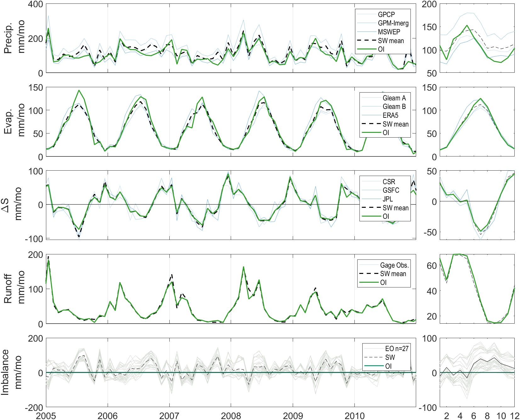
First, let’s look at how much we have changed the observations in each dataset with OI over the gaged basins. We can look at this information in a number of ways, each of which tells a different story about the data. Time series plots are perhaps the most intuitive. Figure 3.15 shows a set of plots for one of our 2,056 river basins. The data is for the White River at Petersburg, Indiana, United States, with a drainage area of 29,000 km². While no river basin is typical, this location does a good job demonstrating the output from our calculations as it has a long record of river discharge. The corrections made in this basin are relatively modest; over this region of the eastern United States, remote sensing datasets tend to be more reliable and well-calibrated due to the density and availability of in situ calibration data.
The analysis covers the 20-year period from 2000–2019, but we’ve zoomed in to a 6-year period to show more detail. The small plots on the right show the seasonality, or the monthly average of each variable. We can see that the simple weighted average (in black) tends to be in the middle of the EO variables (in gray). The OI solution tends to be close to SW, but slight perturbations have been applied. The changes are greater in months where there is a larger imbalance (bottom plots). With the standard OI algorithm, which I refer to here as “strict OI,”, the Imbalance is always zero. For the OI solution with the relaxation factor, the Imbalance is not always zero, but it is much closer to zero than the imbalance calculated with uncorrected EO datasets. Thus, we see that OI has done exactly what we expect, which is to balance the water budget without departing too much from the values in the original EO datasets.
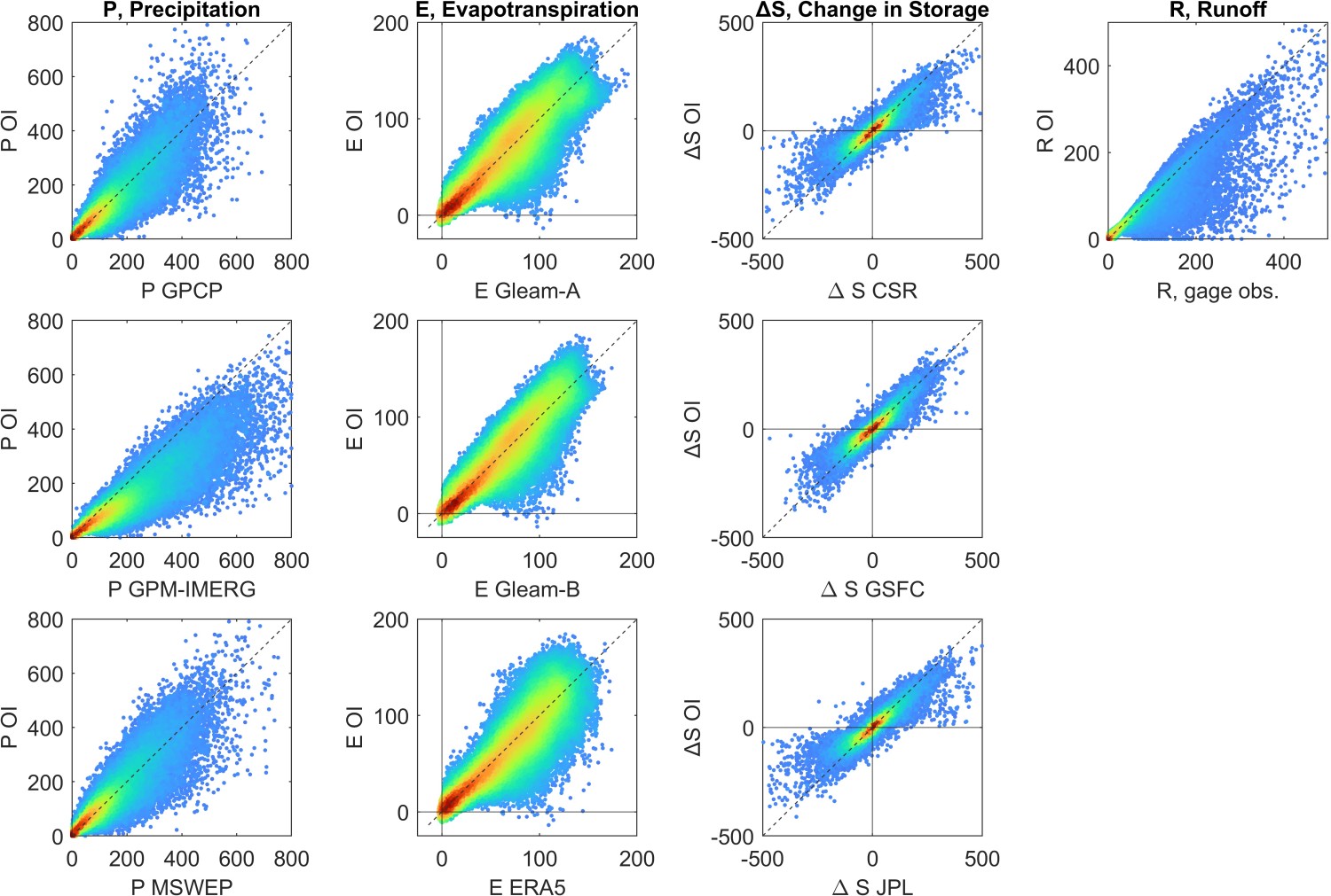
Next, we will look more globally at the changes that OI has made to the input data. Figure 3.16 shows a set of scatter plots, one for each EO input variable. The horizontal axes of each plot shows the uncorrected EO data. For example, in the first plot on the top left, the x-axis is for precipitation estimated by GPCP. The vertical axis is the OI solution for each water cycle component. In the first column, the data for the y-axis is the same for all three plots, because there is a single OI solution for P. The plots are for all months and all 2,056 basins (286,518 paired observations in total, with the color scale indicating greater density of points). We see that the majority of points are clustered around the 1:1 line, indicating that the adjustments made by OI are usually small ones. However, the cloud of points is also quite large, indicating that sometimes OI is making large adjustments to individual components in order to close the water cycle. Here, OI is imposing a strong constraint, and occasionally large corrections are necessary. However, it is reassuring to know that such major corrections are relatively rare. Keep in mind that this is not an exercise in model fitting, where we are trying to maximize \(R^2\). We set out to make modifications to the datasets, and these plots show the extent to which the observations have been modified.
The scatter plots in Figure 3.16 show the relationship between the inputs and the targets for the modeling methods to be described in the following section, Chapter 4. These methods will allow us to make corrections similar to OI, but can be made in ungaged basins, or where input data are incomplete.
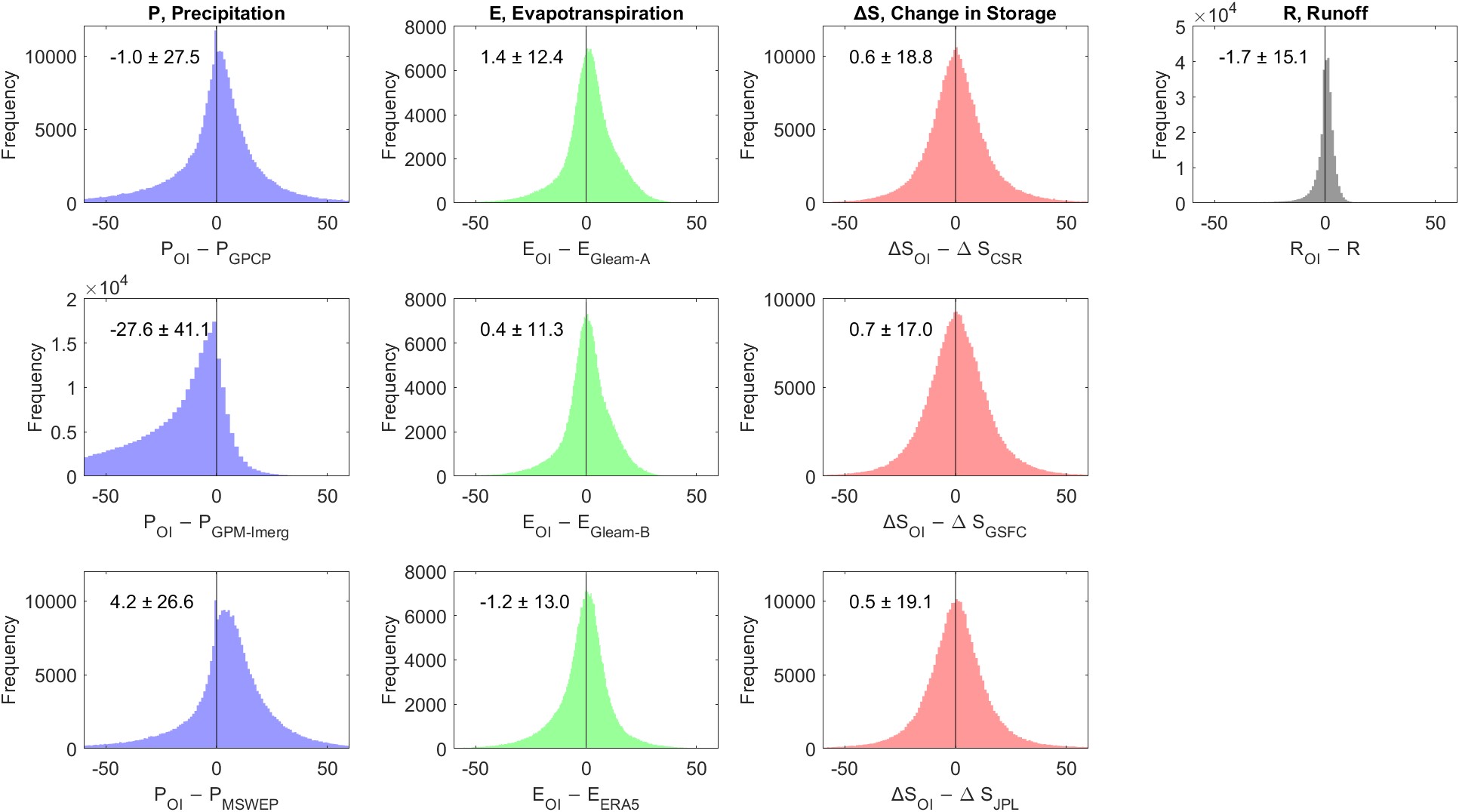
Among the precipitation datasets, OI is making the largest changes to the GPM-IMERG dataset, with a root mean square difference (RMSD) of 49.8 mm/month. Figure 3.17 shows distributions of the changes made to each dataset by OI. The figures also report the mean and standard deviation for each dataset. The average change is typically rather small, around 1 mm/month. The exception again is the dataset GPM-IMERG, where the OI solution is 27.6 mm/month higher, on average.
Finally, we may look at the geographic distribution of the changes OI makes to the datasets. Figure 3.18 shows the average difference between the simple weighted average of the EO datasets and the OI solution for each of the four water cycle components in each of the 2,056 basins. The average difference, equivalent to a bias when we are discussing model error, is calculated between the two time series as the mean of \(\delta^i\) over all time steps i, where \(\delta^i = P_{OI}^i - P_{SW}^i\) for all time steps i. Figure 3.18(a) shows the average corrections made by OI over the gaged basins, while part (b) shows the same over our synthetic river basins, where we are using runoff estimated by GRUN.
In Figure 3.18, each basin is mapped at its centroid, or approximate geographic center. Blue dots mean that \(\delta > 0\), or the OI solution is higher on average than the SW mean, and red means that OI is lower than SW. We see that the OI solution for P is lower than SW over much of the globe. This means that observed precipitation is biased high, and that we have to revise P downward in order to close the water cycle. This is consistent with our previous observation that one of our datasets, GPM-IMERG, consistently overestimates P over much of the globe. The corrections by OI are especially strong over parts of South America, the southern United States, India, and northern Australia. Corrections made to the other three water cycle components are lower in magnitude. Yet, distinct regional patterns emerge. There is a fairly consistent pattern over North America as we move from the northwest to the southeast. In the areas around Alaska and British Columbia, E is adjusted downward, and in the eastern and southern United States, E tends to be adjusted upward. Similar west to east patterns are apparent in South America and South Asia. Changes to runoff tend to be clustered in a few areas, most of which have colder climates. This is likely due to the influence of snow melt that contributes to runoff, and which may be inadequately quantified by GRACE.
We note largely the same patterns between (a) gaged basins and (b) synthetic basins. It is immediately apparent that the spatial coverage of the synthetic basins is much better. Indeed, this is one of the key motivations for working with this data. Nevertheless, in areas where both datasets have coverage, we see some differences. In particular, OI has adjusted runoff upwards in northeastern South America, while the changes made by OI to observed runoff is the opposite. We also see some differences in the changes made to evapotranspiration over South America. A thorough comparison is not possible because of the difference in spatial coverage between the two datasets.
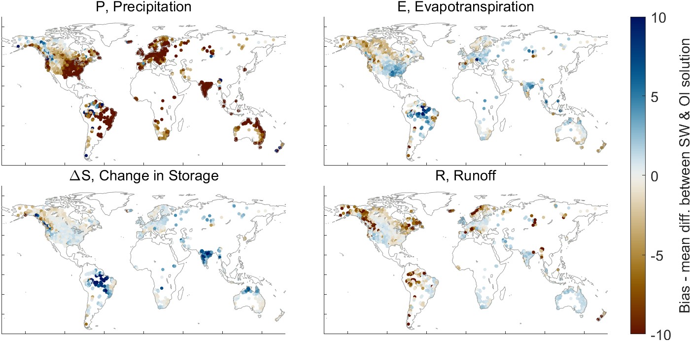
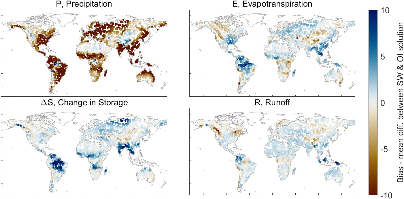
This chapter described methods for combining remote sensing datasets to create a balanced water budget over river basins. I described methods for creating accurate river basin boundaries using topographic data, and for calculating spatial averages of gridded EO variables over the basin boundaries. Preliminary analysis of the EO data showed that there are serious inconsistencies among datasets, as there are large residuals to the water budget equation \(P = E - \Delta S - R\).
I applied the optimal interpolation (OI) method over a collection of over 1,600 basins, a much larger number than previous studies using similar methods. The OI method leverages information from multiple satellite datasets, which may vary in accuracy by season or by location. This takes advantage of the idea that each dataset provides valuable information. Because the hydrologic conditions vary dramatically over the basins, I used a novel affine error model to make OI more flexible and return more realistic results. Maps of the difference between the EO datasets and the OI solution (Figure 3.18) can help illuminate areas where EO variables are less accurate and may need more detailed calibration.
Applying the OI method over thousands of watersheds is already a significant result. To my knowledge, this is the first study to apply these methods over such a large collection of river basins.
The OI method, despite its strengths, has certain limitations. OI imposes a very strong constraint, forcing closure of the water cycle by distributing the water balance residual. Any errors in one measurement will tend to propagate and infect the other components. Furthermore, it can only be applied over river basins, where we have access to river discharge data. One of the goals of this research was to find a method of optimizing EO variables at the pixel scale. In the following chapter, I describe modeling methods to extend the OI solution to the pixel scale.