Wikipedia has thousands of articles about rivers. What are the most important facts about a river? Some can be described with numbers, such as its length, width, or average flow.
I think that every Wikipedia article about a river should include a watershed map. A map can tell you so much, including the landscape features that affect a river’s flow and water quality.
You can make a high-quality map using the free Global Watersheds web app. It is fast and easy. The best part is that you can include a link to a live, interactive map. Below is an example, followed by step-by-step instructions.
You can now delineate watersheds that drain to a polyline or polygon feature. This is useful for finding the total drainage area for a section of coastline or for an inland lake — also known as “endorheic” lakes.
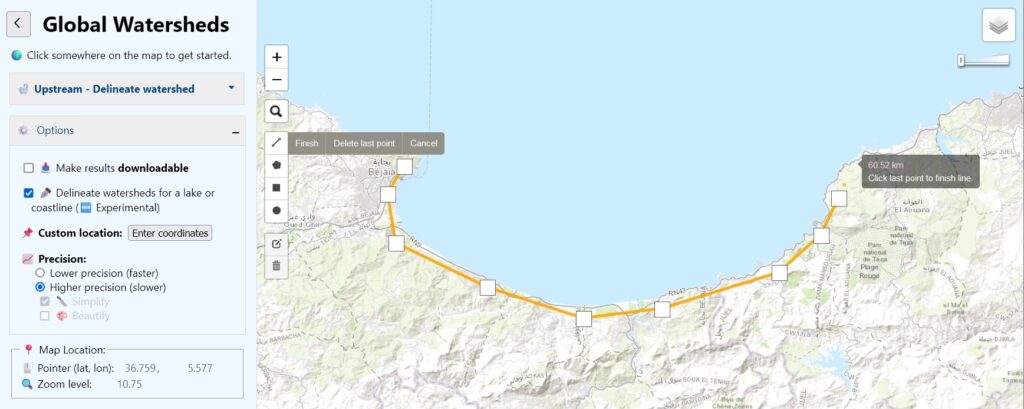
To use this feature, under Options, check the box for Delineate watersheds for a lake or coastline. On the left side of the map, you will see a new drawing toolbar. Select one of the drawing tools, and create a polyline, polygon, rectangle or circle. You can only draw one feature at a time. There are also little buttons to edit your feature or to delete it. Then click on the feature and then click the button Delineate! This feature is only available using MERIT data (not HydroSHEDS), and only in “lower-resolution” mode.
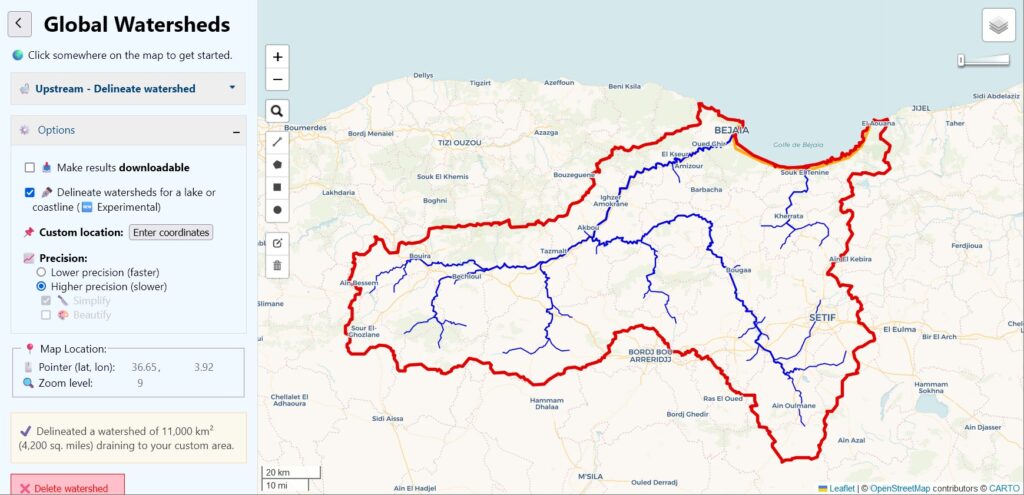
In the example below, I found the area that drains to the Gulf of Bejaia on the Mediterranean coast in Algeria, by drawing a line over the land near the coast:
The resulting drainage area includes two larger rivers or “wadis,” as well as many smaller coastal drainages.
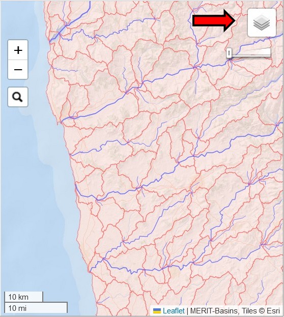
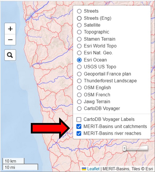
The second new feature allows you to view the MERIT-Basins layers on the map. There are separate layers for “river reaches” and “unit catchments.” These are the data layers that the app uses to construct watersheds when you choose “MERIT” as your data source. To activate these layers, just click on these new layers. They are overlays, which will display on top of your chosen basemap.
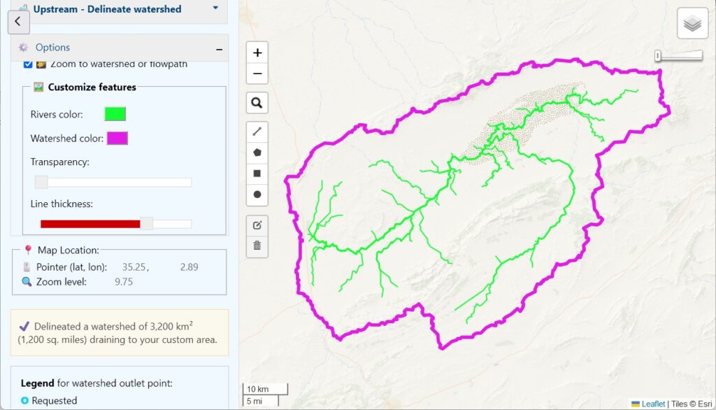
Finally, a small but fun new feature: you can now change the color of your rivers and watershed boundaries. You’ll find the color selectors near the bottom of the Options pane on the left. I’m not sure this is very useful, but you can create some interesting effects:
Please let me know what you think of these new features. Did you find any bugs? How could you use them?
In this post, I’ll give a short tutorial for how to calculate the average precipitation over a watershed or river basin. This is a common task in hydrology and environmental science.
Historically, hydrologists used data from rain gages, which report precipitation at a single location. Yet, everyone knows that rainfall varies a lot from one place to another. So for a large watershed, you might have gathered data from several gages. Hydrologists have developed several clever methods for averaging point observations from multiple gages.
Today, gridded climate data are widely available. For precipitation, gridded data can give you much more information about how rainfall varies with geography. Also, they can give you information for remote or sparsely populated regions where rain gauges are scarce.
If you’re in the US, you might be using PRISM, which is based on a sophisticated interpolation of data from hundreds of gages. Or you could be using a global dataset based on satellite remote sensing, for example CMORPH. If you are looking back at history and need long records, you might choose output from a reanalysis model like NCEP or ERA5.
Below, I show how to calculate the spatial mean of these data. I use precipitation as an example, but the same methods will work with any kind of gridded environmental data – evaporation, temperature, land use, vegetative cover, etc. I’m also talking about watersheds, but the same methods could be used to get the average over a city, a province, the boundaries of a bioregion, etc.
If you only need to do this calculation once, you can use GIS to calculate a zonal average. I’ll show how to do it with the free software QGIS. If you need to do this calculation many times (i.e. with daily precipitation), you will want to write code to automate this. I’ll show how to do that in a future post.
Example Application: Flooding on the Winooski River
Here, we’ll estimate the amount of rain that fell over the Winooski River watershed in Vermont on July 11, 2023, a day where there was major flooding. Here are the steps:
1. Get PRISM precipitation
Go to https://prism.oregonstate.edu/. There are lots of different options. I downloaded provisional daily precipitation for July 11, 2023. Here’s what it looked like:
Unzip the files to a convenient location. The data are in BIL format. This is an old ESRI format for aerial photos and remote sensing data, but it shouldn’t pose a problem if you have a full installation of QGIS.
I panned and zoomed until I found where the Winooski drains to Lake Champlain.
Under Options, check the box for “Make results downloadable.”
Click on the map then click “Delineate!” button in the map popup. Or you can click “Enter coordinates” and enter 44.53, -73.27. It should look something like this:
If the results don’t look right, click in a slightly different location and try again.
On the left of the page, scroll down. Under Downloads, click Watershed Boundary. Click the button to download the watershed boundary. I recommed choosing a GeoPackage, but the other formats will work fine too.
3. Create a map in QGIS
Open QGIS, and create a new project.
Add the watershed: Select Layer > Add layer > Add vector layer, then choose the watershed layer.
Add the precipitation layer: Select Layer > Add layer > Add raster layer, then choose the PRISM precip. layer. Choose the .bil file.
Here, I adjusted the Symbology of the layers to make them look nice.
Use the “Identify features” tool to check a few values of the precip. We can see a pixel in the center of the watershed where the precip was 95 mm on July 11. That is about 3.7 inches. A lot of rain in 24 hours!
4. Calculate the basin average
Open the Toolbox It looks like a little gear in the menu bar, or choose Processing > Toolbox.
Search for the tool Zonal Statistics, and double click it to open. We have to make the right selections in the window that pops up:
Under Input layer, select the watershed vector layer.
Under Raster layer, choose the PRISM precipitation raster.
Under Raster band, keep the default, Band 1. (This raster only has one band. Sometimes a raster will have multiple bands. For example, an image will have separate bands for Red, Green, and Blue.)
Under Statistics to calculate, make sure Mean is included.
Near the bottom, you can keep [Create temporary layer], or you can choose to save the results. Your choices are a variety of geodata layers. Since the results will be a table (not geodata), I chose .csv, a comma-delimited text file.
Click Run.
In a moment, you should see a new table appear in your map’s Table of Contents. Right click on it and choose Open Table.
Note that the table has only one row. That is because our input vector file only had a single feature.
In the table,-mean is 56. That means the watershed received an average of 56 mm of precipitation that day. The field _count has a value of 176. That means that QGIS averaged the value of 176 pixels that itersect our watershed.
Next Steps
That’s it! Now you know how to calculate the average precipitation over a watershed. This kind of calculation is extremely important in many areas of science and engineering. It’s useful for analyzing floods and droughts, in water budget studies, etc.
The approach we used required a lot of clicking. If you need to do it over and over, you can write some code to automate the calculation. Let me know if you’re interested in seeing this in a future post.
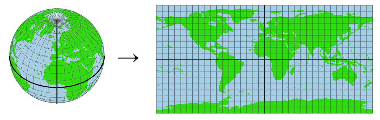
Important note: This method, using the zonal average in GIS, works well when your watershed is small. That is because the pixels all have roughly the same area. If you are dealing with a large watershed, the results will not be accurate, because the area of the pixels varies a lot with latitude. This illustration shows how grid cells get much smaller toward the poles.
For larger watersheds, you should calculate a weighted average that accounts for the varying area of the pixels. This means you’ll have to write some code to do it.
It seems that a few people are discovering the mghydro watershed delineation API. Last Monday, the API handled requests for 9,679 watersheds over the course of a few hours. (Someone is very interested in the watersheds of France!)
One way to use the API is with GIS software, to fetch watershed boundaries and river centerlines from the web app and display them in your desktop GIS. Another use is to automate your requests, rather than using the online map interface. This could be useful if you want to delineate hundreds (or thousands!) of watersheds. However, remember that the results of automated delineation are very often wrong, so you should visually check each one.
Here is a demo in Python of how you could use the API to download watersheds for multiple outlet points. Click on the filename at the bottom to go to Github, where you can download the Jupyter notebook.
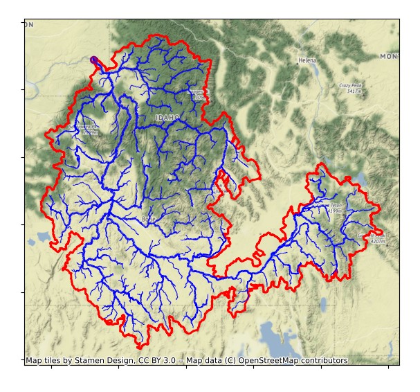
I recently tried my hand at using NLDI, the new water data web service from the U.S. Geological Survey. The service provides access to water data from the National Hydrography Dataset (NHD), version 2. I was specifically interested in using the NHD geodata to delineate watersheds. This data was digitized from 1:100,000-scale maps. (There is newer, more detailed data, called NHDPlus HR, for high-resolution, but no web service for these data yet.)
Snake River watershed upstream of the Lower Granite Dam in eastern Washington state (just a location I picked at random for this demo!)
It took me a couple days of tinkering to get the results I wanted, but the results look impressive and seem accurate. You can run the code yourself by downloading one of these files from GitHub Gists. (Or follow along below.)